Regression trees DAAG Chapter 11 Learning objectives In this - PowerPoint PPT Presentation
Regression trees DAAG Chapter 11 Learning objectives In this section, we will learn about regression trees. What is a regression tree? What types of problems can be addressed with regression trees? How complex a tree? Choosing
Regression trees DAAG Chapter 11
Learning objectives In this section, we will learn about regression trees. ◮ What is a regression tree? ◮ What types of problems can be addressed with regression trees? ◮ How complex a tree? ◮ Choosing the number of splits ◮ Pruning ◮ Random forests
Decision trees Spam email example with 6 explanatory variables: 1. crl.tot (total length of words in capitals) 2. dollar (percentage of characters that are $) 3. bang (percentage of characters that are !) 4. money (percentage of words that are ’money’) 5. n000 (percentage of words with 000) 6. make (percentage of words that are ’make’) There are actually many more variables that were omitted.
Decision trees
Trees are a very flexible tool Types of problems that can be addressed: 1. Regression with a continous response 2. Regression with a binary response 3. Classification with ordered outcomes 4. Classification with unordered outcomes 5. Survival analysis, etc. Trees are best for large datasets with unknown structure. ◮ Make very weak assumptions ◮ Have low power to detect
Spam example 3.5 2.0 ● 2.0 ● ● ● ● ● 8000 3.0 ● 8 1.5 ● 1.5 1.5 2.5 ● ● ● 6000 ● ● ● ● ● ● 6 ● ● ● ● 2.0 ● ● ● ● ● 1.0 ● ● ● ● 1.0 1.0 ● ● ● ● ● 4000 ● ● ● ● ● 1.5 ● ● ● ● ● 4 ● ● ● ● ● ● ● ● ● ● ● ● ● ● ● ● ● ● ● ● ● ● ● ● ● ● ● 1.0 ● ● ● ● ● ● ● ● ● ● ● ● ● ● ● ● ● ● ● 0.5 ● ● ● 2000 0.5 ● ● ● 0.5 ● ● ● ● ● ● ● ● ● ● ● ● ● ● ● ● ● 2 ● ● ● ● ● ● ● ● ● ● ● ● ● 0.5 ● ● ● ● ● ● ● ● ● ● ● ● ● ● ● ● ● ● ● ● ● ● ● ● ● ● ● ● ● ● ● ● ● ● ● ● ● ● ● ● ● ● ● ● ● ● ● ● ● ● ● ● ● ● ● ● ● ● ● ● ● ● ● ● ● ● ● ● ● ● ● ● ● ● ● ● ● ● ● ● ● ● ● ● ● ● ● ● ● ● ● ● ● ● ● ● ● ● ● ● ● ● ● ● ● ● ● ● ● ● ● ● ● ● ● ● ● ● 0.0 ● ● ● ● ● ● ● ● ● ● ● ● ● ● ● ● 0.0 ● 0.0 ● 0.0 ● ● ● ● ● ● ● ● ● ● ● ● ● ● ● ● ● ● ● ● ● ● ● ● ● ● ● ● ● ● ● ● ● 0 ● ● ● ● ● ● 0 ● ● ● ● ● ● ● ● ● ● ● ● ● ● ● ● ● ● ● ● ● ● ● n y n y n y n y n y n y Total runs $ bang money 000 make of capitals ● ● ● ● ● ● 2 ● ● ● ● ● ● ● ● ● ● ● ● ● 5 ● 1000 ● 2 ● ● ● ● (Logarithmic scales) ● ● ● ● ● 1 ● ● ● 1 ● ● ● 1 ● ● ● ● ● ● ● ● ● ● ● ● ● 200 ● ● ● ● ● ● ● ● ● ● ● 2 1 ● ● ● ● ● ● ● ● ● ● ● ● ● ● ● ● ● 0.5 ● 0.5 0.5 ● ● 50 ● ● ● ● ● ● ● ● ● ● ● ● 1 0.5 ● ● ● ● ● ● 20 ● ● ● ● ● ● ● ● ● ● ● ● 0.5 ● ● ● ● ● ● ● ● ● ● ● ● ● ● ● ● ● ● ● ● ● ● ● ● ● ● ● ● ● ● ● ● ● ● ● ● ● 5 ● ● ● ● ● ● 0.1 ● ● 0.1 0.1 ● ● ● ● ● ● ● ● ● ● ● ● 0.1 ● ● ● ● ● ● ● ● ● ● 0.1 ● ● ● ● ● ● ● ● ● ● ● ● ● ● ● ● ● ● ● ● ● ● ● ● ● ● ● ● ● ● ● ● ● ● ● ● ● ● ● ● ● ● ● ● ● ● ● ● ● ● ● ● ● ● ● ● ● ● 1 ● ● n y n y n y n y n y n y Total runs $ bang money 000 make of capitals
Spam example: output Classification tree: rpart(formula = yesno ~ crl.tot + dollar + bang + money + n000 + make, data = spam7, method = "class") Variables actually used in tree construction: [1] bang crl.tot dollar Root node error: 1813/4601 = 0.39404 n= 4601 CP nsplit rel error xerror xstd 1 0.476558 0 1.00000 1.00000 0.018282 2 0.075565 1 0.52344 0.54661 0.015380 3 0.011583 3 0.37231 0.38886 0.013477 4 0.010480 4 0.36073 0.39051 0.013500 5 0.010000 5 0.35025 0.38334 0.013398
Splitting rules ◮ Minimize deviance (residual sum of squares) ◮ Choose the split that results in the smallest possible deviance ◮ Minimize Gini index � k p 2 j � = k p ij p ik = 1 − � ik ◮ leaf i , number of observations in category k is n ik ◮ p ik = n ik / � i n ik ◮ Minimize information criterion D i = � k n ik log( p ik ) ◮ Often additional rules are imposed such as a minimum leaf group size
Determining tree size ◮ We can grow the tree indefinitely because each split will (generally) improve the fit ◮ Need some way to determine when to stop ◮ Cross validation ◮ Complexity parameter ( c p ) trades off complexity (cost) with improved fit (large c p , small tree) ◮ c p is a proxy for the number of splits ◮ Fit a tree that is more complex than optimal ◮ Prune the tree back to achieve an optimal tree by setting c p and minimizing the cross-validated relative error ◮ Rule of thumb: minimum error + 1 standard deviation
Optimal spam tree ◮ Previous c p table had minimum c p = 0 . 01 Classification tree: rpart(formula = yesno ~ crl.tot + dollar + bang + money + n000 + make, data = spam7, method = "class") Variables actually used in tree construction: [1] bang crl.tot dollar Root node error: 1813/4601 = 0.39404 CP nsplit rel error xerror xstd 1 0.476558 0 1.00000 1.00000 0.018282 2 0.075565 1 0.52344 0.54661 0.015380 3 0.011583 3 0.37231 0.38886 0.013477 4 0.010480 4 0.36073 0.39051 0.013500 5 0.010000 5 0.35025 0.38334 0.013398
Optimal spam tree Classification tree: rpart(formula = yesno ~ crl.tot + dollar + bang + money + n000 + make, data = spam7, method = "class", cp = 0.001) Variables actually used in tree construction: [1] bang crl.tot dollar money n000 Root node error: 1813/4601 = 0.39404 n= 4601 CP nsplit rel error xerror xstd 1 0.4765582 0 1.00000 1.00000 0.018282 2 0.0755654 1 0.52344 0.54992 0.015414 3 0.0115830 3 0.37231 0.38389 0.013406 4 0.0104799 4 0.36073 0.37728 0.013310 5 0.0063431 5 0.35025 0.36569 0.013139 6 0.0055157 10 0.31660 0.35135 0.012921 7 0.0044126 11 0.31109 0.33922 0.012732 8 0.0038610 12 0.30667 0.33039 0.012590 *min+1se* 9 0.0027579 16 0.29123 0.32101 0.012436 *min* 10 0.0022063 17 0.28847 0.32377 0.012482 11 0.0019305 18 0.28627 0.32432 0.012491 12 0.0016547 20 0.28240 0.32874 0.012563 13 0.0010000 25 0.27413 0.33039 0.012590
Random forests ◮ Large number of bootstrap samples are used to grow trees independently ◮ Grow each tree by: ◮ Taking a bootstrap sample of the data ◮ At each node, a subset of the variables are selected at random. The best split on this subset is used to split the node. ◮ There is no pruning. Trees are limited by a minimum size at terminal nodes and/or the maximum number of total nodes ◮ Out-of-bag prediction for each observation is done by majority vote across trees that didn’t include that sample ◮ Tuning parameter: the number of variables that are randomly sampled at each split
Single trees vs random forests ◮ Random forests do not provide a unique tree - the entire forest is used for classification by majority vote ◮ Single trees require specification of a unique model matrix ◮ Very little tuning in random forests ◮ Cost parameter controls complexity of single tree ◮ Accuracy for complex data sets can be much better using a random forest ◮ Random forests are much more computationally expensive
Random spam forest Call: randomForest(formula = yesno ~ ., data = spam7, importance = TRUE) Type of random forest: classification Number of trees: 500 No. of variables tried at each split: 2 OOB estimate of error rate: 11.8% Confusion matrix: n y class.error n 2647 141 0.05057389 y 402 1411 0.22173194
Recommend
More recommend
Explore More Topics
Stay informed with curated content and fresh updates.
