Trees Applied Multivariate Statistics Spring 2012 Overview - PowerPoint PPT Presentation
Trees Applied Multivariate Statistics Spring 2012 Overview Intuition for Trees Regression Trees Classification Trees 1 Idea of Trees: Regression Trees Continuous response Binary Tree y Y=1.2 X 1 X>1 Y=1.4 Y=0.7 2 X
Trees Applied Multivariate Statistics – Spring 2012
Overview Intuition for Trees Regression Trees Classification Trees 1
Idea of Trees: Regression Trees Continuous response Binary Tree y Y=1.2 X ≤ 1 X>1 Y=1.4 Y=0.7 2 X > 2 X ≤ 0.3 X > 0.3 X ≤ 2 Y=1.9 Y=0.2 Y=0.3 1 Y=1.3 0 1 2 x 2
Idea of Trees: Classification Tree Discrete response No Yes Survived in Titanic? 800/200 No Sex=F Sex=M 150/50 650/150 No No Age ≥ 27 Age <27 Age ≥ 35 Age <35 3/17 147/33 70/130 580/20 Yes No Yes No Missclassification rate: - Total: (3+33+70+20) / 1000 = 0.126 - “Yes” -class: 53/200 = 0.26 - “No” -class: 73/800 = 0.09 3
Intuition of Trees: Recursive Partitioning For simplicity: Restrict to recursive binary splits 4
Fighting overfitting: Cost-complexity pruning Overfitting: Fitting the training data perfectly might not be good for predicting future data Test error In practice: Use cross-validation Training error Complexity of model For trees: 1. Fit a very detailed model 2. Prune it using a complexity penalty to optimize cross-validation performance 5
Building Regression Trees 1/2 Assume given partition of space R 1 , …, R M Tree model: Goal is to minimize sum of squared residuals: (𝑧 𝑗 − 𝑔 𝑦 𝑗 2 ) Solution: Average of data points in every region 6
Building Regression Trees 2/2 Finding the best binary partition is computationally infeasible Use greedy approach: For variable j and split point s define the two generated regions: Choose splitting variable j and split point s that solve: inner minimization is solved by Repeat splitting process on each of the two resulting regions 7
Pruning Regression Trees Stop splitting when some minimal node size (= nmb. of samples per node) is reached (e.g. 5) Then, cut back the tree again (“pruning”) to optimize the cost-complexity criterion: “Impurity measure” Goodness of fit Complexity Tuning parameter 𝛽 is chosen by cross-validation 8
Classification Trees Regression Tree: Quality of split measured by “Squared error” Classification Tree: Quality of split measured by general “Impurity measure” 9
Classification Trees: Impurity Measures Proportion of class k observations in node m: Define majority class in node m: k(m) Common impurity measures 𝑅 𝑛 (𝑈) : For just two classes: 10
Example: Gini Index Side effects after treatment? 100 persons, 50 with and 50 without side effects: 50 / 50 (No / Yes) Split on age Split on sex 50 / 50 50 / 50 F old young M 30 / 40 20 / 10 10 / 50 40 / 0 Gini = 0.49 Gini = 0.44 Gini = 0.27 Gini = 0 Total Gini = 0.49 + 0.44 = Total Gini = 0.27 + 0 = = 0.93 = 0.27 0.27 < 0.93, therefore: Choose split on age 11
Classification Trees: Impurity Measures Usually: - Gini Index used for building - Misclassification error used for pruning 12
Example: Pruning using Misclass. Error (MCE) 50 / 50 50 / 50 young young old old 10 / 50 40 / 0 10 / 50 40 / 0 MCE = 0.167 MCE = 0 MCE = 0.167 MCE = 0 tall short 0 / 50 10 / 0 MCE = 0 MCE = 0 e.g., 𝛽 = 0.5 𝐷 𝛽 𝑈 = 50 ∗ 0 + 10 ∗ 0 + 40 ∗ 0 + 0.5 ∗ 3 = 𝐷 𝛽 𝑈 = 60 ∗ 0.167 + 40 ∗ 0 + 0.5 ∗ 2 = = 1.5 = 11. 0 Smaller 𝐷 𝛽 (𝑈) , therefore don’t prune 13
Trees in R Function “ rpart ” (recursive partitioning) in package “ rpart ” together with “print”, “plot”, “text” Function “ rpart ” automatically prunes using optimal 𝜷 based on 10-fold CV Functions “ plotcp ” and “ printcp ” for cost -complexity information Function “prune” for manual pruning 14
Concepts to know Trees as recursive partitionings Concept of cost-complexity pruning Impurity measures 15
R functions to know From package “ rpart ”: “ rpart ”, “print”, “plot”, “text”, “ plotcp ”, “ printcp ”, “prune” 16
Recommend
More recommend
Explore More Topics
Stay informed with curated content and fresh updates.
