Binary Trees, Heaps Binary Trees, Heaps Binary trees Binary trees - PowerPoint PPT Presentation

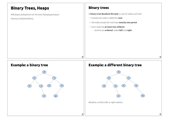
Binary Trees, Heaps Binary Trees, Heaps Binary trees Binary trees A binary tree (δυαδικό δέντρο) is a set of nodes such that: K08 Δομές Δεδομένων και Τεχνικές Προγραμματισμού • Exactly one node is called the root Κώστας Χατζηκοκολάκης • All nodes except the root have exactly one parent • Each node has at most two children - and the are ordered : called left and right / / 1 2 Example: a binary tree Example: a binary tree Example: a di�erent binary tree Example: a di�erent binary tree R R S S T T U V U V X X Y Y W Z Z W Whether a child is left or right matters. / / 3 4

Terminology Terminology Terminology Terminology • path : sequence of nodes traversing from parent to child (or vice-versa) • Nodes tree can be arranged in levels / depths : - The root is at level 0 • length of a path: number of nodes -1 (= number of “moves” it contains) - Its children are at level 1 , their children are at level 2 , etc. • siblings : children of the same parent • Note: node level = length of the (unique) path from the root to that node • descendants : nodes reached by travelling downwards along any path • height of the tree: the largest depth of any node • ancestors : nodes reached by travelling upwards towards the root • subtree rooted at a node: the tree consisting of that node and its • leaf / external node : a node without children descendants • internal node : a node with children / / 5 6 Complete binary trees Complete binary trees Example: complete binary tree Example: complete binary tree A binary tree is called complete (πλήρες) if • All levels except the last are “full” (have the maximum number of nodes) • The nodes at the last level �ll the level “from left to right” / / 7 8

Example: not complete binary tree Example: not complete binary tree Example: not complete binary tree Example: not complete binary tree / / 9 10 Level order Level order Nodes of a complete binary tree Nodes of a complete binary tree Ordering the nodes of a tree level-by-level (and left-to-right in each level). • How many nodes does a complete binary tree have at each level? • At most 1 - 1 0 at level . H - 2 2 1 3 at level . D K - 4 2 at level . - … 6 4 5 7 - 2 k at level . k B F J L 8 9 10 11 12 I C G A E / / 11 12

Properties of binary trees Properties of binary trees Properties of complete binary trees Properties of complete binary trees h ≤ log n • The following hold: h +1 - h + 1 ≤ n ≤ 2 − 1 • Very important property, the tree cannot be too “tall”! - 1 ≤ n ≤ 2 h E • Why? - h ≤ n ≤ 2 − h 1 I - l < h 2 l Any level contains exactly nodes - log( n + 1) − 1 ≤ h ≤ n − 1 - Level contains at least one node h • Where h −1 - 1 + 2 + … + 2 + 1 = 2 ≤ h So n - n : number of all nodes - And take logarithms on both sides - n I : number of internal nodes - n E : number of external nodes (leaves) - h : height / / 13 14 How do we represent a binary tree? How do we represent a binary tree? Sequential representation Sequential representation Store the entries in an array at level order . 1 H 2 3 H D K G B F J L A C E I A: D K 6 7 8 11 1 5 9 10 12 2 3 4 6 4 5 7 • Common for complete trees B F J L • A lot of space is wasted for non-complete trees 8 9 10 11 12 - missing nodes will have empty slots in the array I C G A E / / 15 16

How to �nd nodes How to �nd nodes Heaps Heaps A binary tree is called a heap (σωρός) if To Find: Use Provided A [ i ] A [2 i ] 2 i ≤ n The left child of • It is complete , and A [ i ] A [2 i + 1] 2 i + 1 ≤ n The right child of • each node is greater or equal than its children A [ i ] A [ i /2] i > 1 The parent of A [1] The root is nonempty A (Sometimes this is called a max-heap , we can similarly de�ne a min-heap) A [ i ] 2 i > n Whether is a leaf / / 17 18 Example Example Heaps and priority queues Heaps and priority queues • Heaps are a common data structure for implementing Priority Queues 10 • The following operations are needed 9 8 - �nd max - insert - remove max 5 2 7 6 - create with data • We need to preserve the heap property in each operation! 3 4 1 / / 19 20

Find max Find max Inserting a new element Inserting a new element • Trivial, the max is always at the root • The new element can only be inserted at the end - remember: we always preserve the heap property - because a heap must be a complete tree • Complexity? • Now all nodes except the last satisfy the heap property - to restore it: apply the bubble_up algorithm on the last node / / 21 22 Inserting a new element Inserting a new element Example insertion Example insertion bubble_up(node) • Before - node might be larger than its parent - all other nodes satisfy the heap property • After - all nodes satisfy the heap property • Algorithm - if node > parent ◦ swap them and call bubble_up(parent) / / 23 24

Example insertion Example insertion Example insertion Example insertion Inserting 15 and running bubble_up Inserting 12 and running bubble_up / / 24 24 Complexity of insertion Complexity of insertion Removing the max element Removing the max element • We travel the tree from the last node to the root • We want to remove the root - on each node: 1 step (constant time) - but the heap must be a complete tree O ( h ) • So we need at most steps • So swap the root with the last element - then remove the last element - h is the height of the tree h ≤ log n - but on a complete tree • Now all nodes except the root satisfy the heap property - to restore it: apply the bubble_down algorithm on the root • O (log n ) So - the “complete” property is crucial! / / 25 26

Removing the max element Removing the max element Example removal Example removal bubble_down(node) • Before - node might be smaller than any of its children - all other nodes satisfy the heap property • After - all nodes satisfy the heap property • Algorithm - max_child = the largest child of node - If node < max_child ◦ swap them and call bubble_down(max_child) / / 27 28 Example removal Example removal Complexity of removal Complexity of removal • We travel a single path from the root to a leaf • O ( h ) So we need at most steps - h is the height of the tree • O (log n ) Again - again, having a complete tree is crucial Removing 9 and restoring the heap property / / 28 29

Building a heap from initial data Building a heap from initial data E�cient heapify E�cient heapify • What if we want to create a heap that contains some initial values ? • Better algorithm: - - we call this operation heapify Visit all internal nodes in reverse level order n ◦ last internal node: (parent of the last leaf ) n • “Naive” implementation: 2 ◦ �rst internal node: 1 (root) - Create an empty heap and insert elements one by one - Call bubble_down on each visited node • What is the complexity of this implementation? • Why does this work? - We do inserts n - when we visit node , its subtree is already a heap O (log n ) - Each insert is (because of bubble_up ) ◦ except from node itself (the precondition of bubble_down ) - O ( n log n ) So total - So bubble_down restores the heap property in the subtree • Worst-case example? - After processing the root, the whole tree is a heap - sorted elements: each value with have to fully bubble_up to the root / / 30 31 Heapify example Heapify example Heapify example Heapify example Visit internal nodes in inverse level order, call bubble_down. / / 32 32

Complexity of heapify Complexity of heapify Complexity of heapify Complexity of heapify n • • More careful calculation of the number of steps: We call bubble_down times 2 - h − l If node is at level , bubble_down takes at most steps l O ( n log n ) - So ? 2 l ( h − l )2 l - At most nodes at this level, so steps for level l • But this is only an upper-bound h −1 - ∑ l =0 ( h − l )2 l For the whole tree: - bubble_down is faster closer to the leaves 2 n - This can be shown to be less than (exercise if you're curious) - and most nodes live there! O ( n ) • So we get worst-case complexity - we might be over-approximating the number of steps / / 33 34 E�cient vs naive heapify E�cient vs naive heapify Implementing ADTPriorityQueue Implementing ADTPriorityQueue • O ( n log n ) Types For naive_heapify we found - maybe we are also over-approximating? // Ενα PriorityQueue είναι pointer σε αυτό το struct struct priority_queue { • n log n No: in the worst-case (sorted elements) we really need steps Vector vector; // Τα δεδομένα, σε Vector για μεταβλη CompareFunc compare; // Η διάταξη - try to compute the exact number of steps DestroyFunc destroy_value; // Συνάρτηση που καταστρέφει ένα στοι }; • The di�erence: - bubble_up is faster closer to the root , but few nodes live there - bubble_down is faster closer to the leaves , and most nodes live there • O ( n ) Note: in the average-case , the naive version is also / / 35 36