Learning optimization algorithms with neural networks 1. - PowerPoint PPT Presentation
M.Sc. Data Science thesis presentation - AUEB Nikolaos Stefanos Kostagiolas Supervisor: Prof. Evangelos Markakis Learning optimization algorithms with neural networks 1. Introduction 2. Related Work 3. Meta-learning with recurrent neural
M.Sc. Data Science thesis presentation - AUEB Nikolaos Stefanos Kostagiolas Supervisor: Prof. Evangelos Markakis Learning optimization algorithms with neural networks
1. Introduction 2. Related Work 3. Meta-learning with recurrent neural networks 4. Experiments & Results 5. Conclusion 1 Table of contents
Introduction
Learning: the ability of living organisms to acquire new, or modify existing knowledge, behaviors, skills, values or preferences. Turing: need of a learning mechanism in computer systems as a key element towards emulating human intelligence. Machine Learning : term coined by Arthur Samuel (1959). Formal definition by Tom Mitchell (1998): Machine learning is the study of algorithms that: 2 Origins of machine learning • improve their performance P • at some task T • with experience E Therefore, a well-defined learning task is given by < P , T , E >.
Machine learning is used in settings where: • Human expertise does not exist (navigating on Mars) • Humans can’t explain their expertise (speech recognition - natural language processing) • Models must be customized (personalized medicine) • Models are based on huge amounts of data (genomics) Disclaimer: Machine learning is not a magic wand! 3 Applications of machine learning
sample-efficient: • Kids are able recognize objects easily after being exposed to few examples • People who know how to ride a bike are likely to discover the way to ride a motorcycle fast with little or even no demonstration intelligence” is still the goal). 4 A striking difference from human learning High performance of machine learning model ⇔ abundance of data Machine learning ̸ = human learning, latter is faster and way more Question : is it possible for a machine learning model to exhibit similar properties, i.e. learning new concepts and skills fast with a few training examples? Spoiler : yes indeed (especially if Turing’s ”emulating human
sample efficiency to machine learning algorithms. environments that have never been encountered before during training time exposure to the new task configurations. training examples because its way of learning them is more efficient. Thus it has ”learned to learn”. 5 Solution: ”learning to learn” or simply ”meta-learning” Meta-learning : aims to introduce generalization capabilities and Generalization : the ability of adapting to new tasks and new Adaptation : mini learning session during test time but with limited Profit : The model can complete new tasks without the need of many
6 Visualization example of a meta-learning setting
machine learning problems, e.g. supervised learning, reinforcement learning etc. Examples of meta-learning tasks include: • A classifier trained on non-cat images can tell whether a given image contains a cat after seeing a handful of cat pictures. • A game bot is able to quickly master a new game. • A mini robot completes the desired task on an uphill surface during test even through it was only trained in a flat surface environment. • An optimizer trained on a specific task by a gradient descent variant can perform efficiently tasks of the same family. 7 Application examples More importantly : meta-learning can be applied to a variety of
Related Work
Initial studies in the field of meta-learning: 1990s: • General idea: enhance recurrent neural networks with the ability to modify their own weights. • Downside: high computational requirements! • General idea: Use an LSTM (Long Short-Term Memory) network as an optimizer in order to train multi-layer perceptrons. • General idea: Replace backpropagation with a more biologically-plausible update algorithm 8 Meta-learning: the initial steps • Schmidhuber ’s legacy studies between late 1980s and early • Hochreiter et al. , 2001: • Bengio et al. , 2002:
Despite initial plateaus, meta-learning has become a hot topic within the ML research community with several well known use cases: • Hyper-parameter and neural network optimization, • Deep learning architecture search • Few-shot learning • Speeding-up reinforcement learning 9 Meta-learning: scaling up to form a field during the neural net- work resurgence
General idea instead of devising it. network variant that learns the update rule • Widely applied with general success [1], [2], [3], [4], [5], [6]. • Results in a more efficient update rule than that of a hand-written optimizer (?) while also saving time by bypassing hyperparameter tuning. 10 Approaches to meta-learning: Optimizer learning Work initiated with Hochreiter et al. ’s work discussed earlier • Learn an update rule for the parameters of a neural network • Meta-learner : neural network, typically a recurrent neural • Learner : another network that is updated by the meta-learner. • The meta-learner network acts as the optimizer .
Motivation behind casting optimizer design as a learning problem: existing common elements among the different algorithms used for continuous optimization. • Operation in an iterative fashion where the iterate is a single point in the domain of the objective function. • Random initiation of the iterate point across the domain. • Modification of the iterate at each iteration using a step vector update rule. • An update rule that takes into account the previous or current gradients of the objective function. 11 Approaches to meta-learning: Optimizer learning
Meta-learning with recurrent neural networks
General practice in machine learning: express each task in the form of an optimization problem where the desired outcome is to Usually this is done by applying a form of gradient descent in a sequence of updates of the form: Several optimization algorithms have surfaced in the process, namely momentum, Rprop, Adagrad, RMSprop and ADAM. 12 Problem definition optimize an objective function f ( θ ) over some domain θ ∈ Θ θ t + 1 = θ t − α t ∇ f ( θ t )
exploiting problem-specific structures at the expense of generalization loss function (also referred to as the optimizee) in the following form: Optimizer is constantly informed about the performance of the rule proposals in order to infer the optimal update rule for updating 13 Problem definition Problem : each of the aforementioned algorithms performs well by Solution : learn the update rule by using an optimizer model m φ , specified by parameters φ in order to update the parameters of our θ t + 1 = θ t + g t ( ∇ f ( θ t ) , φ ) optimizee f and, by updating its parameters φ it varies its update the optimizee’s parameters θ , thus maximizing its performance.
14 Intuitive visualization
In our case, the learned update will take the form of a LSTM (a recurrent neural network variant). Why? gradient descent is, at its very essence, a sequence of updates on separate states in-between. that occurred during the optimization process in order to shape better future update rules. architecture that allows information from earlier points in time to persist to later ones. 15 Architecture details • Requirement #1 : a sequential learning architecture is required - • Reason for requirement #1 : reasoning about previous events • Architectural solution #1 : employ a recurrent neural network
But why do we specifically need LSTMs instead of a plain recurrent neural network? has to affect later ones but it also has to be maintained. suggested updates of our optimizer affected the performance of the optimizee has to be accessed in some way. network (or simply LSTM) with a memory-like feature called the cell state . • Disclaimer: Not novel ideas, introduced earlier mainly by 16 Architecture details • Requirement #2 : information about previous states, not only • Reason for requirement #2 : information regarding how previous • Architectural solution #2 : employ a Long Short-Term Memory Andrychowicz et al. , 2016 and widely-applied later.
17 So how is the optimizer trained? • But what if we wanted to relate the expected loss with respect are the optimizer parameters and f is the function we are trying to optimize (or simply the optimizee). • Thus, the expected loss with relation to the optimizer can be written as: state at time t can be denoted as h t . • As it is already mentioned, our LSTM optimizer network m Learning phase details • Let the final optimizee parameters be written as θ ∗ ( f , φ ) where φ [ ] L ( φ ) = E f ← f ( θ ∗ ( f , φ )) − D where f is drawn according to some distribution D of functions . outputs the update steps g t and is parameterized by φ , while its to the parameter values throughout the whole optimization trajectory ?
18 where f efficiently. g t T The previous expected loss definition is equal to the following: Learning phase details [ ] ∑ L ( φ ) = E f w t f ( θ t ) t = 1 θ t + 1 = θ t + g t [ ] = m ( ∇ t , h t , φ ) h t + 1 We can, thus, perform gradient descent on φ in order to minimize L ( φ ) which should give us an optimizer that is capable of optimizing
Basically this is nothing we wouldn’t expect: the loss of the The optimizer takes in the gradient of the optimizee as well as its previous state, and outputs a suggested update that we hope will reduce the optimizee’s loss as fast as possible. 19 Learning phase details optimizer neural net (i.e. our LSTM) is simply the summed training loss of the optimizee as it is trained by the optimizer.
Experiments & Results
Recommend
More recommend
Explore More Topics
Stay informed with curated content and fresh updates.
