Introduction to R Nishant Gopalakrishnan, Martin Morgan 19-21 - PDF document

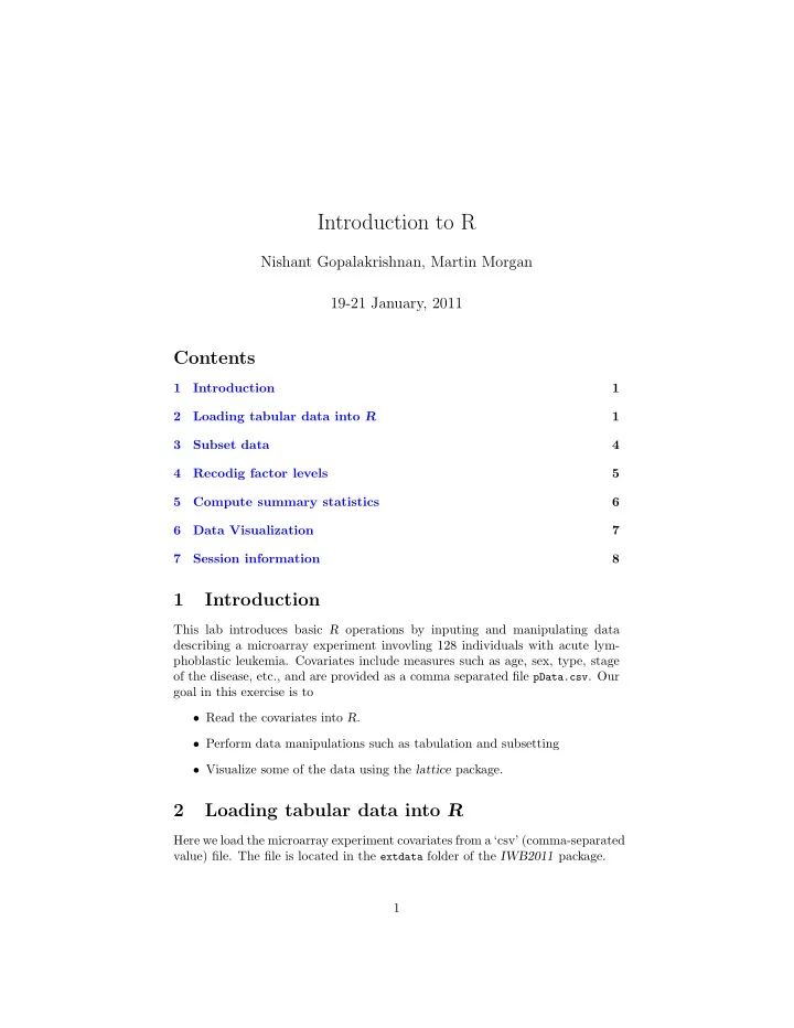
Introduction to R Nishant Gopalakrishnan, Martin Morgan 19-21 January, 2011 Contents 1 Introduction 1 2 Loading tabular data into R 1 3 Subset data 4 4 Recodig factor levels 5 5 Compute summary statistics 6 6 Data Visualization 7 7 Session information 8 1 Introduction This lab introduces basic R operations by inputing and manipulating data describing a microarray experiment invovling 128 individuals with acute lym- phoblastic leukemia. Covariates include measures such as age, sex, type, stage of the disease, etc., and are provided as a comma separated file pData.csv . Our goal in this exercise is to • Read the covariates into R . • Perform data manipulations such as tabulation and subsetting • Visualize some of the data using the lattice package. 2 Loading tabular data into R Here we load the microarray experiment covariates from a ‘csv’ (comma-separated value) file. The file is located in the extdata folder of the IWB2011 package. 1

R provides several functions such as read.table for reading in meta data files into a data.frame with appropriate column and row names from the header information provided in the file. Convenience functions such as count.fields are also available for discovering problems in files (such as certain rows in the file having different number of fields) when using the read.table function. Exercise 1 • Start R, and load the IWB2011 pacakge. • Use the system.file to locate the path to the files exprsMat.csv and pData.csv • Make use of the count.fields function on the pData.csv file to ensure that the file has the same number of fields in each line of the file. • Use the read.table function to read in the experimental meta data into an R variable pdOrig . • View the first few records of the data using head . • Obtain a brief summary of the data using summary . • Tabulate the number of males and females in the study by selecting the sex column and using table . Solution: > library(IWB2011) > phenoPath <- system.file( "extdata", "pData.csv", package="IWB2011") > pdOrig <- read.table(phenoPath) > names(pdOrig) [1] "cod" "diagnosis" "sex" [4] "age" "BT" "remission" [7] "CR" "date.cr" "t.4.11." [10] "t.9.22." "cyto.normal" "citog" [13] "mol.biol" "fusion.protein" "mdr" [16] "kinet" "ccr" "relapse" [19] "transplant" "f.u" "date.last.seen" > head(pdOrig) cod diagnosis sex age BT remission CR date.cr 01005 1005 5/21/1997 M 53 B2 CR CR 8/6/1997 01010 1010 3/29/2000 M 19 B2 CR CR 6/27/2000 03002 3002 6/24/1998 F 52 B4 CR CR 8/17/1998 04006 4006 7/17/1997 M 38 B1 CR CR 9/8/1997 04007 4007 7/22/1997 M 57 B2 CR CR 9/17/1997 04008 4008 7/30/1997 M 17 B1 CR CR 9/27/1997 2

t.4.11. t.9.22. cyto.normal citog mol.biol 01005 FALSE TRUE FALSE t(9;22) BCR/ABL 01010 FALSE FALSE FALSE simple alt. NEG 03002 NA NA NA <NA> BCR/ABL 04006 TRUE FALSE FALSE t(4;11) ALL1/AF4 04007 FALSE FALSE FALSE del(6q) NEG 04008 FALSE FALSE FALSE complex alt. NEG fusion.protein mdr kinet ccr relapse transplant 01005 p210 NEG dyploid FALSE FALSE TRUE 01010 <NA> POS dyploid FALSE TRUE FALSE 03002 p190 NEG dyploid FALSE TRUE FALSE 04006 <NA> NEG dyploid FALSE TRUE FALSE 04007 <NA> NEG dyploid FALSE TRUE FALSE 04008 <NA> NEG hyperd. FALSE TRUE FALSE f.u date.last.seen 01005 BMT / DEATH IN CR <NA> 01010 REL 8/28/2000 03002 REL 10/15/1999 04006 REL 1/23/1998 04007 REL 11/4/1997 04008 REL 12/15/1997 > summary(pdOrig) cod diagnosis sex age 10005 : 1 1/15/1997 : 2 F :42 Min. : 5.00 1003 : 1 1/29/1997 : 2 M :83 1st Qu.:19.00 1005 : 1 11/15/1997: 2 NA ' s: 3 Median :29.00 1007 : 1 2/10/1998 : 2 Mean :32.37 1010 : 1 2/10/2000 : 2 3rd Qu.:45.50 11002 : 1 (Other) :116 Max. :58.00 (Other):122 NA ' s : 2 NA ' s : 5.00 BT remission CR B2 :36 CR :99 CR :96 B3 :23 REF :15 DEATH IN CR : 3 B1 :19 NA ' s:14 DEATH IN INDUCTION: 7 T2 :15 REF :15 B4 :12 NA ' s : 7 T3 :10 (Other):13 date.cr t.4.11. t.9.22. 11/11/1997: 3 Mode :logical Mode :logical 1/21/1998 : 2 FALSE:86 FALSE:67 10/18/1999: 2 TRUE :7 TRUE :26 12/7/1998 : 2 NA ' s :35 NA ' s :35 1/17/1997 : 1 3

(Other) :87 NA ' s :31 cyto.normal citog mol.biol Mode :logical normal :24 ALL1/AF4:10 FALSE:69 simple alt. :15 BCR/ABL :37 TRUE :24 t(9;22) :12 E2A/PBX1: 5 NA ' s :35 t(9;22)+other:11 NEG :74 complex alt. :10 NUP-98 : 1 (Other) :21 p15/p16 : 1 NA ' s :35 fusion.protein mdr kinet ccr p190 :17 NEG :101 dyploid:94 Mode :logical p190/p210: 8 POS : 24 hyperd.:27 FALSE:74 p210 : 8 NA ' s: 3 NA ' s : 7 TRUE :26 NA ' s :95 NA ' s :28 relapse transplant f.u Mode :logical Mode :logical REL :61 FALSE:35 FALSE:91 CCR :23 TRUE :65 TRUE :9 BMT / DEATH IN CR: 4 NA ' s :28 NA ' s :28 BMT / CCR : 3 DEATH IN CR : 2 (Other) : 7 NA ' s :28 date.last.seen 1/7/1998 : 2 12/15/1997: 2 12/31/2002: 2 3/29/2001 : 2 7/11/1997 : 2 (Other) :83 NA ' s :35 > table(pdOrig$sex) F M 42 83 3 Subset data The pdOrig variable is a data.frame with columns representing the various co- variates that describe the experiment (age, sex, etc.). The row names correspond 4

to the sample Id’s. The column BT is a factor indicating the tumour cell type (B1, B2, T1 ,T2 etc. with B indicating B-cell type and T indicating T-cell type). Similarly the column mol biol is a factor indicating the molecular biol- ogy of the cancer. (BCR/ABL, NEG, E2A/PBX1 etc.) The mol biol column can be accessed using pdOrig[["mol biol"]] . In this section, we make use of indexing, subsetting, factors etc. to modify pdOrig to select a subset of samples. We are specifically interested in B-cell tumours with molecular biology type ”NEG” or ”BCR/ABL”. Exercise 2 • Identify the samples that are ”NEG” or ”BCR/ABL” molecular biology type using the column mol biol , the %in% function and the which functions in R. • Use the grep function on the BT column in the pdOrig data.frame to identify the B cell tumours. • Identify samples that are both B cell tumours and are ”BCR/ABL” or ”NEG”using the intersect function on the indices that we have previously computed. • Subset the phenotypic data pdOrig to create a new variable psubData . Note:The rows of the data.frame represent samples. Solution: > types <- c("NEG", "BCR/ABL") > moltyp <- which(as.character(pdOrig$mol.biol) %in% types) > bcell <- grep("^B", as.character(pdOrig$BT)) > indx <- intersect(bcell, moltyp) > psubData <- pdOrig[indx,] 4 Recodig factor levels The covariate data for some variables, for example BT , is represented using a variable of type factor. The ‘levels’ are the distinct categorical values of a factor. Subsetting a factor leaves the levels of the variable unchanged. In this exercise, we take a look at the levels of the factor variables that we have just subsetted, and then update the levels. Exercise 3 • Observe the levels for the mol.biol and moltyp variables Do you notice any problem ?. • Recode the factor levels for the mol.biol and moltyp variables using the factor function. 5

Solution: > levels(psubData$BT) [1] "B" "B1" "B2" "B3" "B4" "T" "T1" "T2" "T3" "T4" > psubData$BT <- factor(psubData$BT) > levels(psubData$BT) [1] "B" "B1" "B2" "B3" "B4" > psubData$mol.biol <- factor(psubData$mol.biol) > levels(psubData$mol.biol) [1] "BCR/ABL" "NEG" 5 Compute summary statistics R includes several functions that allows you to do a lot while writing only few lines of code. A good example is the aggregate function that splits the data into subsets, computes summary statistics for each subset, and returns the result in a convenient form. For more details regarding this function, please type in help("aggregate") into an R session. We will be making use of the formula and the data.frame methods for the aggregate function in this example. Another useful function for creating contingency tables that we will be using is the xtabs function. We proceed to create some summary statistics on the variable psubData using the aggregate and xtabs functions. Exercise 4 • Find the average age of male and females in our subsetted metadata vari- able psubData for the NEG and BCR/ABL groups using the data.frame interface for the aggregate function. The table generated by using the aggregate should look similar to the one found below. Hint: Try passing na.rm = TRUE to the aggregate function sex molBiol age 1 F BCR/ABL 39.94 2 M BCR/ABL 40.50 3 F NEG 29.75 4 M NEG 24.86 • Recalculate the average age of male and females in our subsetted metadata variable psubData for the NEG and BCR/ABL groups, this time using the formula interface for the aggregate function. Make sure that the results are identical to the one from the previous step. 6