Introduction to Matlab with mathematical and engineering - PowerPoint PPT Presentation

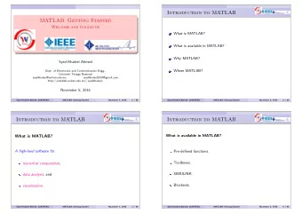
Introduction to Matlab with mathematical and engineering applications Hanumant Singh Shekhawat Indian Institute of Technology Guwahati India April 11,2015 (IITG, India) April 11,2015 1 / 30

Objective Learning basic Matlab with some elementary engineering and mathematical applications (IITG, India) April 11,2015 2 / 30

Outline Outline 1 Round off error 2 Matrices 3 Basic Numerical Mathematics 4 Ordinary differential equations (IITG, India) April 11,2015 3 / 30

Round off error Round off error • Define variable x = 1 − 1 / 3 − 2 / 3. • Theoretically x = 0 • check using x == 0 • What do you get ? and why ? (IITG, India) April 11,2015 4 / 30

Matrices Different data types (IITG, India) April 11,2015 5 / 30

Matrices Linear equations • Consider the following linear equation 3 x 1 + 4 x 2 = 1 x 2 = 2 x 1 + x 3 = 0 • The above is equivalent to Ax = B   3 4 0 � T and  , B = � where 3 × 3 matrix A = 0 1 0 1 2 0  1 0 1 � T � x = x 1 x 2 x 3 • x = A − 1 B • The matrix notation is useful in solving large number of equations. (IITG, India) April 11,2015 6 / 30

Matrices Solving linear equation   3 4 0  in Matlab as • Define a 3 × 3 matrix A = 0 1 0  1 0 1 � � A = 3 4 0; 0 1 0; 1 0 1 � T (Matlab: � • Solve for x in Ax = B where vector B = 1 2 0 � ′ ). � B = 1 2 0 • x = A − 1 B (in Matlab: x = inv ( A ) ∗ B ) (IITG, India) April 11,2015 7 / 30

Matrices Solving linear equation in a faster way   3 4 0  in Matlab as • Define a 3 × 3 matrix A = 0 1 0  1 0 1 � � A = 3 4 0; 0 1 0; 1 0 1 � T (Matlab: • Solve for x in Ax = B where vector B = � 1 2 0 � ′ ) � 1 2 0 B = • Matlab: x = A \ B • The time difference is visible in case of a large size matrix. • N = 1500; • A = rand ( N , N ); • B = rand ( N , 1); • tic; inv ( A ) ∗ B ; toc • tic; A \ B ; toc (IITG, India) April 11,2015 8 / 30

Matrices Least square solution of a linear equation   3 4  in Matlab as • Define a 3 × 2 matrix A = 0 1  1 0 � � A = 3 4; 0 1; 1 0 � T (Matlab: � • Solve for x in Ax = B where vector B = 1 2 0 � ′ ) � B = 1 2 0 • Theory: No solution • Matlab: x = A \ B . You will get an answer !! • Matlab gives the least square solution • x minimizes � y − B � 2 = � 3 1 ( y i − B i ) 2 where y = Ax (IITG, India) April 11,2015 9 / 30

Matrices Many solutions of a linear equation � 3 � 4 0 • Define a 2 × 3 matrix A = in Matlab as 1 0 1 � � A = 3 4 0; 1 0 1 � T (Matlab: • Solve for x in Ax = B where vector B = � 1 2 � ′ ). � 1 2 B = • Matlab: x = A \ B • Obtain y = null ( A ); • Check x + λ y is also a solution of Ax = B . • Which solution to use in case of many solutions? (IITG, India) April 11,2015 10 / 30

Matrices Exercise Let continuous function f : [ − 1 1] → R be unknown. However, we have r measurements of it, say at x 1 , · · · , x r . Find an approximation f r (it is a continuous function) such that � f − f r � minimized at the �� r i =1 ( f ( x i ) − f r ( x i )) 2 . measurement point i.e. minimize • Out of many methods we choose the 3rd order polynomial approximation i.e. f r ( x ) = a 0 + a 1 x + a 2 x 2 + a 3 x 3 • let the measurement is given by f ( x i ) = cos ( x i ) + sin ( x i ) 3 ; x i = i ∗ 0 . 01; for i = 0 , 1 , · · · 100. • In reality, we just have data points f ( x i ) instead of an equation. • Use f ( x i ) = f r ( x i ) to generate 101 equation. Use matrices here otherwise you will waste a lot of time and paper . � � • Find the least square solution a = a 0 a 1 a 2 a 3 • Plot f ( x i ) and f r ( x i ). (IITG, India) April 11,2015 11 / 30

Matrices Advance Exercises Repeat the last exercise with the following approximations: • Higher order polynomial approximation ? Do you observe singularity ? • Legendre polynomials approximation 3 x 2 − 1 5 x 3 − 3 x f r ( x ) = a 0 + a 1 x + a 2 + a 3 2 2 Do you observe any advantage over polynomials? • Fourier approximation f r ( x ) = a 0 + a 1 cos (2 π x ) + a 2 cos (4 π x ) + a 3 cos (6 π x ) • Which one gives a better approximation ? (IITG, India) April 11,2015 12 / 30

Matrices Eigenvalue decomposition   10 12 1 • Define a 3 × 3 matrix A = 12 17 0   1 0 1 • Calculate A 3 . • Now represent A as A = MDM − 1 (the eigenvalue decomposition ) where D is a diagonal matrix (non-zero entries on the diagonal only). Here use [ M , D ] = eig ( A ) in Matlab. • A 3 = MD 3 M − 1 . Which one is easy to compute? • Check the above in Matlab. • Take any colom of M (say x ) and calculate y = Ax . • Divide first entry of y with first entry of x . Repeat for second and third. • Did you get same result ? • Coloms of M are eigenvectors and diagonal entries of D are called eigenvalues. (IITG, India) April 11,2015 13 / 30

Matrices Singular value decomposition (SVD) • Matrix A can be written as A = UDV T where D has entries (known as singular values ) only along the diagonal and UU T = VV T = I . I is the identity matrix. • Matlab • A= rand(3,2); • [ U , D , V ] = svd ( A ); • UU T = I and VV T = I (size of I may change) • Get size of all matrices. • Get eigenvalue decomposition of AA T and A T A . • Do you see U and V there ? • Any relationship between D here and the eigenvalues of AA T and A T A . (IITG, India) April 11,2015 14 / 30

Matrices Image Download the image from http://img1.jurko.net/wall/uploads/wallpaper_13409.jpg and save as ’end.jpeg’. (IITG, India) April 11,2015 15 / 30

Matrices Image Download the image from http://img1.jurko.net/wall/uploads/wallpaper_13409.jpg and save as ’end.jpeg’. Use the following commands to read the image in Matlab as a matrix • X = imread(’end.jpeg’,’jpg’); • X = rgb2gray(X); • image(X) • colormap(gray(256)) X is a matrix of size 600 × 800 (IITG, India) April 11,2015 16 / 30

Matrices Image compression • Compression means reducing the memory requirement to store the data. • Image is a matrix M = UDV T (SVD). • One method of image compression is to replace smaller singular values with zero. DV T where ˜ • ˜ M = U ˜ D is the same matrix as D except that it contains only the r largest singular values (the other singular values are replaced by zero). • � M − ˜ M � F = � D − ˜ D � F . Here � . � just means root mean square of all entries of the matrix. • Try this for a random matrix A = rand (4 , 4). • Why this is a compression ? (IITG, India) April 11,2015 17 / 30

Matrices Exercise (Image compression) • Download the image from http: //img1.jurko.net/wall/uploads/wallpaper_13409.jpg and save as ’end.jpeg’. • Matlab: X = imread(’end.jpeg’,’jpg’); • Matlab: X = rgb2gray(X); • Matlab: image(X) • Matlab: colormap(gray(256)) • Compute the SVD of X, using the command: [U,D,V] = svd(X); • Retain only k = 50 singular values and make the rest zero. • Try with k equal to 100, 150, 200. • What do you observe ? • Calculate compression ratio ? • Plot the singular values (divided by the largest) on the semi-log scale. (IITG, India) April 11,2015 18 / 30

Matrices Advance Exercises • How many singular values are sufficient for an approximation ? • Divide the image in four equal pieces and do an approximation of all four images. Now join them together. Is this method gives you good result ? (IITG, India) April 11,2015 19 / 30

Basic Numerical Mathematics Fixed points • Define variable x 0 = 100. • Find x 1 using iterations x n +1 = cos( x n ) • Repeat 30 times to get x 30 . • Did you get 0 . 73908 · · · ? why ? • Repeat with x 0 = 0 • Repeat with x 0 = 9 e 6 • 0 . 73908 · · · is a fixed point of iterations x n +1 = cos( x n ) and is a solution of x = cos( x ). Why ? • No dynamics at the fixed point ! • Can you write a program without worrying of number of repetitions to get a fixed point? • In general, all solutions of x = f ( x ) are called fixed points. (IITG, India) April 11,2015 20 / 30

Basic Numerical Mathematics Fixed points, contd • Define variable x 0 = 0 . 673. • Find x 1 using iterations x n +1 = x 2 n • Repeat 20 times to get x 20 . • Did you get 0 ? why ? • Repeat with x = 1 • Repeat with x = 1 . 000001 and x = 0 . 999999 • Slight change in 1 and we are away from 1. • 1 is an unstable fixed point of iterations x n +1 = x 2 n . • Repeat with x = 1 e − 6 and x = − 1 e − 6 • Slight change in 0 and we are on 0 again. • 0 is a stable fixed point of iterations x n +1 = x 2 n . (IITG, India) April 11,2015 21 / 30

Basic Numerical Mathematics Discrete time system • A discrete time system (zero-input) is defined by an iteration or difference equation x k +1 = f ( x k ) , k = 1 , 2 , · · · where f : R n → R n . • x is called fixed point of discrete time system x k +1 = f ( x k ) if x = f ( x ) • Loosely speaking stability of a fixed point x means that a variation in x will lead iteration x k +1 = f ( x k ) to x . (IITG, India) April 11,2015 22 / 30