Informed Search Chapter 4 Adapted from materials by Tim Finin, - PowerPoint PPT Presentation
Artificial Intelligence Informed Search Chapter 4 Adapted from materials by Tim Finin, Marie desJardins, and Charles R. Dyer Today s Class Iterative improvement methods Hill climbing Simulated annealing Local beam search
Artificial Intelligence Informed Search Chapter 4 Adapted from materials by Tim Finin, Marie desJardins, and Charles R. Dyer
Today ’ s Class • Iterative improvement methods – Hill climbing – Simulated annealing – Local beam search • Genetic algorithms • Online search These approaches start with an initial guess at the solution and gradually improve until it is one.
Hill climbing on a surface of states Height Defined by Evaluation Function
Hill-climbing search • Looks one step ahead to determine if any successor is better than the current state; if there is, move to the best successor. • Rule: If there exists a successor s for the current state n such that • h ( s ) < h ( n ) and • h ( s ) ≤ h ( t ) for all the successors t of n , then move from n to s . Otherwise, halt at n . • Similar to Greedy search in that it uses h (), but does not allow backtracking or jumping to an alternative path since it doesn ’ t “ remember ” where it has been. • Corresponds to Beam search with a beam width of 1 (i.e., the maximum size of the nodes list is 1). • Not complete since the search will terminate at "local minima," "plateaus," and "ridges."
Hill climbing example 2 8 3 2 1 3 start 1 6 4 8 4 h = 0 goal h = -4 7 5 7 6 5 -2 -5 -5 2 8 3 2 1 3 h = -3 1 4 8 4 h = -1 7 6 5 7 6 5 -3 -4 2 2 3 3 h = -2 1 8 4 1 8 4 7 6 5 7 6 5 h = -3 -4 f ( n ) = -(number of tiles out of place)
Exploring the Landscape local maximum • Local Maxima : peaks that aren ’ t the highest point in the plateau space • Plateaus: the space has a broad flat region that gives the search algorithm no direction (random walk) • Ridges: flat like a plateau, but ridge with drop-offs to the sides; steps to the North, East, South Image from: http://classes.yale.edu/fractals/CA/GA/Fitness/Fitness.html and West may go down, but a step to the NW may go up.
Drawbacks of hill climbing • Problems: local maxima, plateaus, ridges • Remedies: – Random restart: keep restarting the search from random locations until a goal is found. – Problem reformulation: reformulate the search space to eliminate these problematic features • Some problem spaces are great for hill climbing and others are terrible.
Example of a local optimum 1 2 5 f = -7 7 4 move start goal up 8 6 3 1 2 5 1 2 3 8 7 4 8 4 f = 0 move 6 3 7 6 5 right 1 2 5 f = -6 f = -7 8 7 4 f = -(manhattan distance) 6 3
Gradient ascent / descent Images from http://en.wikipedia.org/wiki/Gradient_descent • Gradient descent procedure for finding the arg x min f(x) – choose initial x 0 randomly – repeat • x i+1 ← x i – η f ' (x i ) – until the sequence x 0 , x 1 , …, x i , x i+1 converges • Step size η (eta) is small (perhaps 0.1 or 0.05)
Gradient methods vs. Newton ’ s method • A reminder of Newton ’ s method from Calculus: x i+1 ← x i – η f ' (x i ) / f '' (x i ) • Newton ’ s method uses 2 nd order information (the second derivative, or, curvature) to take a more direct route to the minimum. Contour lines of a function • The second-order information is Gradient descent (green) more expensive to compute, but Newton ’ s method (red) converges quicker. Image from http://en.wikipedia.org/wiki/Newton's_method_in_optimization
Simulated annealing • Simulated annealing (SA) exploits an analogy between the way in which a metal cools and freezes into a minimum-energy crystalline structure (the annealing process) and the search for a minimum [or maximum] in a more general system. • SA can avoid becoming trapped at local minima. • SA uses a random search that accepts changes that increase objective function f , as well as some that decrease it. • SA uses a control parameter T , which by analogy with the original application is known as the system “ temperature. ” • T starts out high and gradually decreases toward 0.
Simulated annealing (cont.) • A “ bad ” move from A to B is accepted with a probability P(move A → B ) = e ( f (B) – f (A)) / T • The higher the temperature, the more likely it is that a bad move can be made. • As T tends to zero, this probability tends to zero, and SA becomes more like hill climbing • If T is lowered slowly enough, SA is complete and admissible.
The simulated annealing algorithm
Local beam search • Begin with k random states • Generate all successors of these states • Keep the k best states • Stochastic beam search: Probability of keeping a state is a function of its heuristic value
Genetic algorithms • Similar to stochastic beam search • Start with k random states (the initial population) • New states are generated by “ mutating ” a single state or “ reproducing ” (combining via crossover) two parent states (selected according to their fitness) • Encoding used for the “ genome ” of an individual strongly affects the behavior of the search • Genetic algorithms / genetic programming are a large and active area of research
In-Class Paper Discussion Stephanie Forrest. (1993). Genetic algorithms: principles of natural selection applied to computation. Science 261 (5123): 872–878.
Class Exercise: Local Search for Map/Graph Coloring
Online search • Interleave computation and action (search some, act some) • Exploration: Can ’ t infer outcomes of actions; must actually perform them to learn what will happen • Competitive ratio = Path cost found* / Path cost that could be found** * On average, or in an adversarial scenario (worst case) ** If the agent knew the nature of the space, and could use offline search • Relatively easy if actions are reversible ( ONLINE-DFS-AGENT ) • LRTA* (Learning Real-Time A*): Update h ( s ) (in state table) based on experience • More about these issues when we get to the chapters on Logic and Learning!
Summary: Informed search • Best-first search is general search where the minimum-cost nodes (according to some measure) are expanded first. • Greedy search uses minimal estimated cost h ( n ) to the goal state as measure. This reduces the search time, but the algorithm is neither complete nor optimal. • A* search combines uniform-cost search and greedy search: f ( n ) = g ( n ) + h ( n ). A* handles state repetitions and h ( n ) never overestimates. – A* is complete and optimal, but space complexity is high. – The time complexity depends on the quality of the heuristic function. – IDA* and SMA* reduce the memory requirements of A*. • Hill-climbing algorithms keep only a single state in memory, but can get stuck on local optima. • Simulated annealing escapes local optima, and is complete and optimal given a “ long enough ” cooling schedule. • Genetic algorithms can search a large space by modeling biological evolution. • Online search algorithms are useful in state spaces with partial/no information.
Recommend
More recommend
Explore More Topics
Stay informed with curated content and fresh updates.
