Multiple Changepoint Detection in Climate Time Series Robert Lund - PowerPoint PPT Presentation
Introduction Annual New Bedford Precipitations Genetic Algorithms Simulation Study Multiple Changepoint Detection in Climate Time Series Robert Lund Clemson Math Sciences Lund@Clemson.edu Joint work with Shanghong Li, Yingbo Li, and Hewa
Introduction Annual New Bedford Precipitations Genetic Algorithms Simulation Study Multiple Changepoint Detection in Climate Time Series Robert Lund Clemson Math Sciences Lund@Clemson.edu Joint work with Shanghong Li, Yingbo Li, and Hewa Priyadarshani June 13, 2017 Robert Lund Clemson Math Sciences Lund@Clemson.edu Multiple Changepoint Detection in Climate Time Series
Introduction Annual New Bedford Precipitations Genetic Algorithms Simulation Study The Need to Detect Changepoints. Changepoints are discontinuity times (inhomogeneities) in a time series. In climate settings, these can be induced from changes in observation locations, equipment, measurement techniques, environmental changes, etc. In this talk, a changepoint is a time where the mean of the series first undergoes a structural pattern change. Changepoint issues are critical when estimating trends. Many changepoints go undocumented. Changepoint techniques can help calibrate new gauges. Robert Lund Clemson Math Sciences Lund@Clemson.edu Multiple Changepoint Detection in Climate Time Series
Introduction Annual New Bedford Precipitations Genetic Algorithms Simulation Study Tuscaloosa, AL Annual Temperatures 20 Observed Temperature (Degrees Celsius) 19 18 17 16 15 1910 1920 1930 1940 1950 1960 1970 1980 1990 2000 Time of Observation (Year) Robert Lund Clemson Math Sciences Lund@Clemson.edu Multiple Changepoint Detection in Climate Time Series
Introduction Annual New Bedford Precipitations Genetic Algorithms Simulation Study New Bedford, MA Annual Temperatures Observed Temperature (Degrees Celsius) 13 11 9 7 1820 1840 1860 1880 1900 1920 1940 1960 1980 2000 Time of Observation (Year) Yearly Temperatures at New Bedford MA With Least Squares Trends Robert Lund Clemson Math Sciences Lund@Clemson.edu Multiple Changepoint Detection in Climate Time Series
Introduction Annual New Bedford Precipitations Genetic Algorithms Simulation Study Key Questions How many changepoints are there? At what times do the changepoints occur? Some recent penalized likelihood references: 1. Davis, Lee, and Rodriguez-Yam, Journal of the American Statistical Association , (2006). 2. Lu, Lund, and Lee, Annals of Applied Statistics , (2010). 3. Li and Lund, Journal of Climate , (2012). Robert Lund Clemson Math Sciences Lund@Clemson.edu Multiple Changepoint Detection in Climate Time Series
Introduction Annual New Bedford Precipitations Genetic Algorithms Simulation Study Our Model For annual ( T = 1), monthly ( T = 12), or daily ( T = 365) data, our model for the data { X t } N t =1 takes a time series regression: X nT + ν = µ ν + α ( nT + ν ) + δ nT + ν + ǫ nT + ν . The seasonal index ν ∈ { 1 , . . . , T } . µ ν is the seasonal mean at season ν . α is a linear trend parameter, which may or may not be needed. Other trend functions are possible. Robert Lund Clemson Math Sciences Lund@Clemson.edu Multiple Changepoint Detection in Climate Time Series
Introduction Annual New Bedford Precipitations Genetic Algorithms Simulation Study More on the Model For annual ( T = 1), monthly ( T = 12) or daily ( T = 365) data, our model for the data { X t } is a time series regression: X nT + ν = µ ν + α ( nT + ν ) + δ nT + ν + ǫ nT + ν . The mean shifts are parametrized in { δ nT + ν } : ∆ 1 = 0 , 1 ≤ t < τ 1 , ∆ 2 , τ 1 ≤ t < τ 2 , δ t = . . . ∆ m +1 , τ m ≤ t < τ m +1 . The errors { ǫ nT + ν } are a zero mean autoregressive process (this is periodic if T > 1). Robert Lund Clemson Math Sciences Lund@Clemson.edu Multiple Changepoint Detection in Climate Time Series
Introduction Annual New Bedford Precipitations Genetic Algorithms Simulation Study The model for annual data The model for annual data is X t = µ + α t + δ t + ǫ t . Location parameter: µ Linear trend: α t Piecewise constant mean shifts: δ t Stationary but correlated errors { ǫ t } Robert Lund Clemson Math Sciences Lund@Clemson.edu Multiple Changepoint Detection in Climate Time Series
Introduction Annual New Bedford Precipitations Genetic Algorithms Simulation Study Periodic Autoregressions A zero-mean series { ǫ nT + ν } is called a periodic autoregression of order p (PAR( p )) if it satisfies the periodic linear difference equation p � ǫ nT + ν = φ k ( ν ) ǫ nT + ν − k + Z nT + ν . k =1 Here, { Z nT + ν } is zero-mean periodic white noise with Var( Z nT + ν ) = σ 2 ( ν ) > 0 for all seasons ν . φ 1 ( ν ) , . . . , φ p ( ν ) are the PAR coefficients during season ν . Such series are indeed “periodically stationary”. Robert Lund Clemson Math Sciences Lund@Clemson.edu Multiple Changepoint Detection in Climate Time Series
Introduction Annual New Bedford Precipitations Genetic Algorithms Simulation Study Penalized Likelihood Methods A penalized likelihood for our model has form − log( L ∗ ( m , τ 1 , . . . , τ m )) + Penalty( m , τ 1 , . . . , τ m ) . L ∗ ( m , τ 1 , . . . , τ m ) is an optimized model likelihood given the changepoint count m and location times τ 1 < · · · < τ m . Penalty( m , τ 1 , . . . , τ m ) is a penalty for the changepoint configuration. Common Penalty( m ; τ 1 , . . . , τ m ) terms used: AIC = 2 m . BIC = m ln( N ). MDL = � m +1 i =1 ln( τ i − τ i − 1 ) / 2 + ln( m ) + � m i =2 ln( τ i ). Robert Lund Clemson Math Sciences Lund@Clemson.edu Multiple Changepoint Detection in Climate Time Series
Introduction Annual New Bedford Precipitations Genetic Algorithms Simulation Study New Bedford, MA Annual Precipitations New Bedford, MA Annual Precipitation 1900 1700 1500 Annual Precipitation(mm) 1300 1100 900 700 500 1815 1835 1855 1875 1895 1915 1935 1955 1975 1995 Time of observation Robert Lund Clemson Math Sciences Lund@Clemson.edu Multiple Changepoint Detection in Climate Time Series
Introduction Annual New Bedford Precipitations Genetic Algorithms Simulation Study Lognormal Annual Precipitation Setup The logarithm of { X t } is modeled as a Gaussian time series with no trend, multiple mean shifts, and autoregressive errors (AR( p )). Here, T = 1: no periodicities. For each changepoint configuration ( m ; τ 1 , . . . , τ m ), we must Fit a time series model with optimal time series parameters and mean shift sizes. Compute the penalty m +1 m � � MDL( m ; τ 1 , . . . , τ m ) = ln( τ i − τ i − 1 ) / 2+ln( m )+ ln( τ i ) . i =1 i =2 Robert Lund Clemson Math Sciences Lund@Clemson.edu Multiple Changepoint Detection in Climate Time Series
Introduction Annual New Bedford Precipitations Genetic Algorithms Simulation Study Two Segment Models Robert Lund Clemson Math Sciences Lund@Clemson.edu Multiple Changepoint Detection in Climate Time Series
Introduction Annual New Bedford Precipitations Genetic Algorithms Simulation Study Three Segment Models Robert Lund Clemson Math Sciences Lund@Clemson.edu Multiple Changepoint Detection in Climate Time Series
Introduction Annual New Bedford Precipitations Genetic Algorithms Simulation Study Four Segment Models Robert Lund Clemson Math Sciences Lund@Clemson.edu Multiple Changepoint Detection in Climate Time Series
Introduction Annual New Bedford Precipitations Genetic Algorithms Simulation Study Five Segment Models Robert Lund Clemson Math Sciences Lund@Clemson.edu Multiple Changepoint Detection in Climate Time Series
Introduction Annual New Bedford Precipitations Genetic Algorithms Simulation Study Six Segment Models Robert Lund Clemson Math Sciences Lund@Clemson.edu Multiple Changepoint Detection in Climate Time Series
Introduction Annual New Bedford Precipitations Genetic Algorithms Simulation Study Summary The table below shows optimum MDL scores for various numbers of model segments. These values were obtained by exhaustive search and are exact. Table: Optimum MDL Scores # Segments Changepoint Times MDL Score 1 — -296.7328 2 1967 -303.8382 3 1917, 1967 -306.6359 4 1867, 1910, 1967 -309.2878 5 1867, 1910, 1965, 1967 -309.8570 6 1829, 1832, 1867, 1910, 1967 -308.2182 Robert Lund Clemson Math Sciences Lund@Clemson.edu Multiple Changepoint Detection in Climate Time Series
Introduction Annual New Bedford Precipitations Genetic Algorithms Simulation Study The Combinatorial Wall We need to minimize − log( L ∗ ( m , τ 1 , . . . , τ m )) + MDL( m , τ 1 , . . . , τ m ) . over all m and τ 1 , . . . , τ m . An exhaustive search over all models with m changepoints requires � N � evaluation of MDL scores. m Summing this over m = 0 , 1 , . . . , N − 1 shows that an exhaustive optimization requires 2 N − 1 different MDL evaluations. We now devise a genetic algorithm for this. A genetic algorithm is an intelligent random walk search. Robert Lund Clemson Math Sciences Lund@Clemson.edu Multiple Changepoint Detection in Climate Time Series
Introduction Annual New Bedford Precipitations Genetic Algorithms Simulation Study Genetic Algorithms (GAs) Chromosome Representation. Each changepoint configuration has the form ( m ; τ 1 , . . . , τ m ). Selection. Give mating preference to the fittest individuals, allowing them to pass their genes on to the next generation. Fitness is determined by the objective function − log( L ∗ ( m ; τ 1 , . . . , τ m )) + MDL( m ; τ 1 , . . . , τ m ) . Robert Lund Clemson Math Sciences Lund@Clemson.edu Multiple Changepoint Detection in Climate Time Series
Recommend
More recommend
Explore More Topics
Stay informed with curated content and fresh updates.
