Informed search algorithms Outline Best-first search Greedy - PowerPoint PPT Presentation
Informed search algorithms Outline Best-first search Greedy best-first search A * search Heuristics Local search algorithms Hill-climbing search Best-first search Idea: use an evaluation function f(n) for each node
Informed search algorithms
Outline • Best-first search • Greedy best-first search • A * search • Heuristics • Local search algorithms • Hill-climbing search
Best-first search • Idea: use an evaluation function f(n) for each node – estimate of "desirability« -istenme derecesi- Expand most desirable unexpanded node • Implementation: Order the nodes in fringe in decreasing order of desirability • Special cases: – greedy best-first search – A * search
Romania with step costs in km
Greedy best-first search • Evaluation function f(n) = h(n) (heuristic) • = estimate of cost from n to goal • e.g., h SLD (n) = straight-line distance from n to Bucharest • Greedy best-first search expands the node that appears to be closest to goal
Greedy best-first search example
Greedy best-first search example
Greedy best-first search example
Greedy best-first search example
Properties of greedy best-first search • Complete? No – can get stuck in loops, e.g., Iasi Neamt Iasi Neamt • Time? O(b m ) , but a good heuristic can give dramatic improvement • Space? O(b m ) -- keeps all nodes in memory • Optimal? No
A * search • Idea: avoid expanding paths that are already expensive • Evaluation function f(n) = g(n) + h(n) • g(n) = cost so far to reach n • h(n) = estimated cost from n to goal • f(n) = estimated total cost of path through n to goal
A * search example
A * search example
A * search example
A * search example
A * search example
A * search example
Admissible heuristics • A heuristic h(n) is admissible – kabul edilebilir - if for every node n , h(n) ≤ h * (n), where h * (n) is the true cost to reach the goal state from n . • An admissible heuristic never overestimates – fazla tahmin etmez - the cost to reach the goal, i.e., it is optimistic • Example: h SLD (n) (never overestimates the actual road distance) • Theorem: If h(n) is admissible, A * using TREE-SEARCH is optimal
Properties of A* • Complete? Yes (unless there are infinitely many nodes with f ≤ f(G) ) • Time? Exponential • Space? Keeps all nodes in memory • Optimal? Yes
Admissible heuristics E.g., for the 8-puzzle: • h 1 (n) = number of misplaced tiles • h 2 (n) = total Manhattan distance (i.e., no. of squares from desired location of each tile) • h 1 (S) = ? • h 2 (S) = ?
Admissible heuristics E.g., for the 8-puzzle: • h 1 (n) = number of misplaced tiles • h 2 (n) = total Manhattan distance (i.e., no. of squares from desired location of each tile) • h 1 (S) = ? 8 • h 2 (S) = ? 3+1+2+2+2+3+3+2 = 18
Relaxed problems • A problem with fewer restrictions on the actions is called a relaxed problem • The cost of an optimal solution to a relaxed problem is an admissible heuristic for the original problem •
Local search algorithms • In many optimization problems, the path to the goal is irrelevant; the goal state itself is the solution • State space = set of "complete" configurations • Find configuration satisfying constraints, e.g., n-queens • In such cases, we can use local search algorithms • keep a single "current" state, try to improve it
Example: n -queens • Put n queens on an n × n board with no two queens on the same row, column, or diagonal •
Hill-climbing search • "Like climbing Everest in thick fog with amnesia" •
Hill-climbing search • Problem: depending on initial state, can get stuck in local maxima •
Hill-climbing search: 8-queens problem • h = number of pairs of queens that are attacking each other, either directly or indirectly • h = 17 for the above state
Hill-climbing search: 8-queens problem • A local minimum with h = 1
Constraint Satisfaction Problems
Outline • Constraint Satisfaction Problems (CSP) • Backtracking search for CSPs
Constraint satisfaction problems (CSPs) • Standard search problem: • – state is a "black box“ – any data structure that supports successor function, heuristic function, and goal test • CSP: – state is defined by variables X i with values from domain D i – – goal test is a set of constraints specifying allowable combinations of values for subsets of variables • Allows useful general-purpose algorithms with more power than standard search algorithms
Example: Map-Coloring • Variables WA, NT, Q, NSW, V, SA, T • Domains D i = {red,green,blue} • Constraints: adjacent regions must have different colors • • e.g., WA ≠ NT, or (WA,NT) in {(red,green),(red,blue),(green,red), (green,blue),(blue,red),(blue,green)} •
Example: Map-Coloring • Solutions are complete and consistent assignments, e.g., WA = red, NT = green,Q = red,NSW = green,V = red,SA = blue,T = green
Constraint graph • Constraint graph: nodes are variables, arcs are constraints
Real-world CSPs • Assignment problems – e.g., who teaches what class • Timetabling problems • – e.g., which class is offered when and where? • Transportation scheduling • • Factory scheduling • • Notice that many real-world problems involve real-valued variables
Standard search formulation (incremental) Let's start with the straightforward approach, then fix it States are defined by the values assigned so far • Initial state: the empty assignment { } • Successor function: assign a value to an unassigned variable that does not conflict with current assignment fail if no legal assignments • Goal test: the current assignment is complete 1. This is the same for all CSPs 2. Every solution appears at depth n with n variables use depth-first search 3. Path is irrelevant, so can also use complete-state formulation
Backtracking search • Variable assignments are commutative - değişmeli }, i.e., [ WA = red then NT = green ] same as [ NT = green then WA = red ] • It repeatedly chooses an unassigned variable and then tries all values in the domain of that variable in turn, trying to find a solution. • Backtracking search is the basic uninformed algorithm for CSPs
Backtracking search
Backtracking example
Backtracking example
Backtracking example
Backtracking example
Improving backtracking efficiency • General-purpose methods can give huge gains in speed: – Which variable should be assigned next? – In what order should its values be tried? – Can we detect inevitable failure early?
Most constrained variable • Most constrained variable: choose the variable with the fewest legal values • a.k.a. minimum remaining values (MRV) heuristic
Most constraining variable • Most constraining variable: • choose the variable with the most constraints on remaining variables
Least constraining value • Given a variable, choose the least constraining value: – the one that rules out the fewest values in the remaining variables • Combining these heuristics makes 1000 queens feasible
Summary • CSPs are a special kind of problem: – states defined by values of a fixed set of variables – goal test defined by constraints on variable values • Backtracking = depth-first search with one variable assigned per node • Variable ordering and value selection heuristics help significantly
Recommend
More recommend
Explore More Topics
Stay informed with curated content and fresh updates.

