Impact analysis of local atmospheric dynamics to pollution transport - PowerPoint PPT Presentation

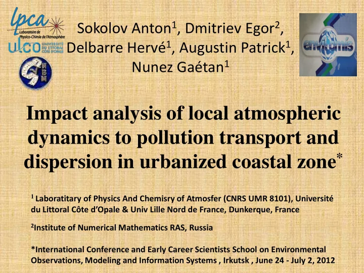
Sokolov Anton 1 , Dmitriev Egor 2 , Delbarre Hervé 1 , Augustin Patrick 1 , Nunez Gaétan 1 Impact analysis of local atmospheric dynamics to pollution transport and dispersion in urbanized coastal zone * 1 Laboratitary of Physics And Chemisry of Atmosfer (CNRS UMR 8101), Université du Littoral Côte d’Opale & Univ Lille Nord de France, Dunkerque, France 2 Institute of Numerical Mathematics RAS, Russia *International Conference and Early Career Scientists School on Environmental Observations, Modeling and Information Systems , Irkutsk , June 24 - July 2, 2012

Plan of the talk • Region of Dunkirk • Measurement campaign BTEX 2006 • Numerical model set-up • Simulations with different resolutions • Backward trajectories • Prespectives and conclusions

Campaign BTEX 2006 Volatile organic compounds Principal sources: (VOC) : • Industry – 36% • benzene • Transport – 32% • Residential - 20 % • toluene • Energy production - 7% • ethylbenzine • Agriculture – 5% • m/p xylene • o xylene Measurements: • at 5 stations • each 15 min • from February till October

Characterization of air mass • age - by concentration ratio, e.g. C(Bz)/C(Tl) • signature of an industry (also by ratio) • localization - by simultaneous peaks of pollution • pollution + windrose: St Pol Port Est N N Bensene NNW NNE 6 NNW NNE NW NE 4 NW NE 4 Toluene NWW NEE NWW NEE 2 2 Ethylbenzene W E 0 W E 0 SWW SEE SWW SEE m,p-Xylene SW SE SW SE SSW SSE o-Xylene SSW SSE S S

Numerical model set-up MESO-NH non-hydrostatic model 3 included models – • Model 1 1500x1500km, 10km • Model 2 120x120km, 2 km • Model 3 35x35km, 0.5 km, 3D turbulence scheme • Z: 70 levels up to 12 km. SURFEX surface scheme , resolution 0.5 km in Europe Two week period in June, 15 min

120 km y Resolution comparison (1) A 15m temperature, horizontal cut, sea breeze A. Model 2 (2 km), which interacts with Model 3 B. Model 3 (resolution 0.5 km) C. Zoom of A correspond to domain of Model 3 120 km x y C B 35 km 35 km x

120 km y Resolution comparison (2) A 15m wind speed, horizontal cut, sea breeze A. Model 2 (2 km), which interacts with Model 3 B. Model 3 (resolution 0.5 km) C. Zoom of A correspond to domain of Model 3 120 km x y C B 35 km 35 km x

120 km y Resolution comparison (3) A wind speed, vertical YZ cut (B, C) , sea breeze A. Model 2 (2 km), which interacts with Model 3 (horizontal cut, 15 m) B. Model 3 (resolution 0.5 km) C. Zoom of A correspond to domain of Model 3 120 km x z z C B 1200 m 1200 m 35 km y 35 km y

Backward trajectories in horizontal (XY) plane (a) 9 June 12:00 - low pollution (b) 13 June 6:00 - high pollution (a) (b) 120 km 120 km 120 km 120 km

Backward trajectories in vertical (YZ) plane (a) 9 June 12:00 - low pollution (b) 13 June 6:00 - high pollution (b) (a) 300 m 300 m 120 km 120 km

Backward trajectories, C(o-Xylene) > 2 µg/m -3 1.Transport pollution (a) 3 2.Industrial pollution (a) 2 3.Port 1 pollution (b) N S a. « Non-local » pollution b. « Local » pollution

Conclusions • COV measurements are coupled with model backward terajectorys • Fine resolution is important • Key role of local atmospheric dynamics (sea and offshore breezes) Perspectives • Cluster analysis • Map of regional pollution • Additional chemical tracers

All the backward trajectoires, model 2 Thank you for your attention!.. )

Trajectoires and centroids (k-means)