Image Segmentation Computer Vision Jia-Bin Huang, Virginia Tech - PowerPoint PPT Presentation

Image Segmentation Computer Vision Jia-Bin Huang, Virginia Tech Many slides from D. Hoiem

Administrative stuffs • HW 3 due 11:59 PM, Oct 17 (Wed) • Final project proposal due Oct 23 (Mon) • Title • Problem • Tentative approach • Evaluation • References

Today’s class • Review/finish Structure from motion • Multi-view stereo • Segmentation and grouping • Gestalt cues • By clustering (k-means, mean-shift) • By boundaries (watershed) • By graph (merging , graph cuts) • By labeling (MRF) <- Next Thursday • Superpixels and multiple segmentations

Perspective and 3D Geometry • Projective geometry and camera models • Vanishing points/lines • x = 𝐋 𝐒 𝐮 𝐘 • Single-view metrology and camera calibration • Calibration using known 3D object or vanishing points • Measuring size using perspective cues • Photo stitching • Homography relates rotating cameras 𝐲′ = 𝐈𝐲 • Recover homography using RANSAC + normalized DLT • Epipolar Geometry and Stereo Vision • Fundamental/essential matrix relates two cameras 𝐲 ′ 𝐆𝐲 = 𝟏 • Recover 𝐆 using RANSAC + normalized 8-point algorithm, enforce rank 2 using SVD • Structure from motion X j • Perspective SfM: triangulation, bundle adjustment • Affine SfM: factorization using SVD, enforce rank 3 x 1 j x 3 j constraints, resolve affine ambiguity x 2 j P 1 P 3 P 2

Review: Projective structure from motion • Given: m images of n fixed 3D points i = 1 ,… , m, j = 1 , … , n x ij = P i X j , • Problem: estimate m projection matrices P i and n 3D points X j from the mn corresponding 2D points x ij X j x 1 j x 3 j x 2 j P 1 P 3 P 2 Slides: Lana Lazebnik

Review: Affine structure from motion • Given: m images and n tracked features x ij • For each image i, c enter the feature coordinates • Construct a 2 m × n measurement matrix D : • Column j contains the projection of point j in all views • Row i contains one coordinate of the projections of all the n points in image i • Factorize D : • Compute SVD: D = U W V T • Create U 3 by taking the first 3 columns of U • Create V 3 by taking the first 3 columns of V • Create W 3 by taking the upper left 3 × 3 block of W • Create the motion (affine) and shape (3D) matrices: ½ V 3 ½ and S = W 3 T A = U 3 W 3 • Eliminate affine ambiguity • Solve L = CC T using metric constraints • Solve C using Cholesky decomposition • Update A and X: A = AC, S = C -1 S Source: M. Hebert

Multi-view stereo

Multi-view stereo: Basic idea Source: Y. Furukawa

Multi-view stereo: Basic idea Source: Y. Furukawa

Multi-view stereo: Basic idea Source: Y. Furukawa

Multi-view stereo: Basic idea Source: Y. Furukawa

Plane Sweep Stereo input image input image reference camera • Sweep family of planes at different depths w.r.t. a reference camera • For each depth, project each input image onto that plane • This is equivalent to a homography warping each input image into the reference view • What can we say about the scene points that are at the right depth? R. Collins. A space-sweep approach to true multi-image matching. CVPR 1996.

Plane Sweep Stereo Scene surface Sweeping plane Image 2 Image 1

Plane Sweep Stereo • For each depth plane • For each pixel in the composite image stack, compute the variance • For each pixel, select the depth that gives the lowest variance • Can be accelerated using graphics hardware R. Yang and M. Pollefeys. Multi-Resolution Real-Time Stereo on Commodity Graphics Hardware , CVPR 2003

Merging depth maps • Given a group of images, choose each one as reference and compute a depth map w.r.t. that view using a multi-baseline approach • Merge multiple depth maps to a volume or a mesh (see, e.g., Curless and Levoy 96) Map 1 Map 2 Merged

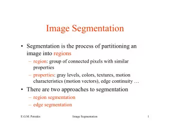
Grouping and Segmentation • Image Segmentation • Which pixels belong together? • Hidden Variables, the EM Algorithm, and Mixtures of Gaussians • How to handle missing data? • MRFs and Segmentation with Graph Cut • How do we solve image labeling problems?

How many people?

Gestalt psychology or gestaltism German: Gestalt - "form" or "whole” Berlin School, early 20th century Kurt Koffka, Max Wertheimer, and Wolfgang Köhler View of brain: • whole is more than the sum of its parts • holistic • parallel • analog • self-organizing tendencies Slide from S. Saverese

Gestaltism The Muller-Lyer illusion

We perceive the interpretation, not the senses

Principles of perceptual organization From Steve Lehar: The Constructive Aspect of Visual Perception

Principles of perceptual organization

Gestaltists do not believe in coincidence

Emergence

Grouping by invisible completion From Steve Lehar: The Constructive Aspect of Visual Perception

Grouping involves global interpretation From Steve Lehar: The Constructive Aspect of Visual Perception

Grouping involves global interpretation From Steve Lehar: The Constructive Aspect of Visual Perception

Gestalt cues • Good intuition and basic principles for grouping • Basis for many ideas in segmentation and occlusion reasoning • Some (e.g., symmetry) are difficult to implement in practice

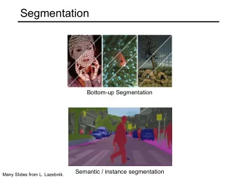
Image segmentation Goal: Group pixels into meaningful or perceptually similar regions

Segmentation for efficiency: “ superpixels ” [Felzenszwalb and Huttenlocher 2004] [Shi and Malik 2001] [Hoiem et al. 2005, Mori 2005]

Segmentation for feature support 50x50 Patch 50x50 Patch

Segmentation for object proposals “Selective Search” [Sande, Uijlings et al. ICCV 2011, IJCV 2013] [Endres Hoiem ECCV 2010, IJCV 2014]

Segmentation as a result Rother et al. 2004

Major processes for segmentation • Bottom-up : group tokens with similar features • Top-down: group tokens that likely belong to the same object [Levin and Weiss 2006]

Segmentation using clustering • Kmeans • Mean-shift

Feature Space Source: K. Grauman

K-means algorithm Partition the data into K sets S = {S 1 , S 2 , … S K } with corresponding centers μ i Partition such that variance in each partition is as low as possible

K-means algorithm Partition the data into K sets S = {S 1 , S 2 , … S K } with corresponding centers μ i Partition such that variance in each partition is as low as possible

K-means algorithm 1.Initialize K centers μ i (usually randomly) 2.Assign each point x to its nearest center: 3.Update cluster centers as the mean of its members 4.Repeat 2-3 until convergence (t = t+1)

function C = kmeans(X, K) % Initialize cluster centers to be randomly sampled points [N, d] = size(X); rp = randperm(N); C = X(rp(1:K), :); lastAssignment = zeros(N, 1); while true % Assign each point to nearest cluster center bestAssignment = zeros(N, 1); mindist = Inf*ones(N, 1); for k = 1:K for n = 1:N dist = sum((X(n, :)-C(k, :)).^2); if dist < mindist(n) mindist(n) = dist; bestAssignment(n) = k; end end end % break if assignment is unchanged if all(bestAssignment==lastAssignment), break; end; % Assign each cluster center to mean of points within it for k = 1:K C(k, :) = mean(X(bestAssignment==k, :)); end end

K-means clustering using intensity alone and color alone Image Clusters on intensity Clusters on color

K-Means pros and cons • Pros – Simple and fast – Easy to implement • Cons – Need to choose K – Sensitive to outliers • Usage – Rarely used for pixel segmentation

Mean shift segmentation D. Comaniciu and P. Meer, Mean Shift: A Robust Approach toward Feature Space Analysis, PAMI 2002. • Versatile technique for clustering-based segmentation

Mean shift algorithm • Try to find modes of this non-parametric density

Kernel density estimation Kernel Estimated density Data (1-D)

Kernel density estimation Kernel density estimation function Gaussian kernel

Mean shift Region of interest Center of mass Mean Shift vector Slide by Y. Ukrainitz & B. Sarel

Mean shift Region of interest Center of mass Mean Shift vector Slide by Y. Ukrainitz & B. Sarel

Mean shift Region of interest Center of mass Mean Shift vector Slide by Y. Ukrainitz & B. Sarel

Mean shift Region of interest Center of mass Mean Shift vector Slide by Y. Ukrainitz & B. Sarel

Mean shift Region of interest Center of mass Mean Shift vector Slide by Y. Ukrainitz & B. Sarel

Mean shift Region of interest Center of mass Mean Shift vector Slide by Y. Ukrainitz & B. Sarel

Mean shift Region of interest Center of mass Slide by Y. Ukrainitz & B. Sarel

Computing the Mean Shift Simple Mean Shift procedure: • Compute mean shift vector • Translate the Kernel window by m(x)     2 n x - x      i x g   i   h    i 1     m x ( ) x   2   n x - x    i g     h      i 1 Slide by Y. Ukrainitz & B. Sarel

Real Modality Analysis