Segmentation H. Papasaika, E. Baltsavias Image Segmentation - PowerPoint PPT Presentation
Segmentation H. Papasaika, E. Baltsavias Image Segmentation Partitioning of an image into a set of regions Regions representing meaningful areas of the image, such as crops, urban areas, forests. Various applications in Computer
Segmentation H. Papasaika, E. Baltsavias
Image Segmentation Partitioning of an image into a set of regions Regions representing meaningful areas of the image, such as crops, urban areas, forests. Various applications in Computer Vision and Geomatics. “What is interesting and what is not” depends on the application.
What defines an object? "I stand at the window and see a house, trees, sky. Theoretically I might say there were 327 brightnesses and nuances of colour. Do I have "327"? No. I have sky, house, and trees." -- Max Wertheimer Max Wertheimer
Gestalt Theory Gestalt theory: psychological theory of vision emphasizing how relations between visual objects affects their perception Principle of Similarity : similar elements are seen as a group Basic image Nearness Color similarity Shape similarity Common behavior
Image segmentation Haralick and Shapiro: The regions should be uniform uniform and homogeneous homogeneous with respect to some characteristic such as intensity value, color or texture. Region interiors should be simple simple and without many small holes holes . Adjacent regions should have significantly different different values with respect to the characteristic on which they values are uniform. Boundaries of each segment should be simple simple , not ragged , and must be spatially accurate. ragged Achieving all is difficult, and in some cases requiring high- level knowledge
Image Segmentation Segmentation is based on two basic properties of values (here grey level): Discontinuity , i.e. to partition the image based on abrupt changes in intensity (grey levels), e.g. edges Similarity , i.e. to partition the image into similar (according to predefined criteria) regions
Edge detection before segmentation Edge detection Edge detection is a useful first step toward image segmentation, but not adequate by itself Ideal case: Segmentation techniques detecting intensity discontinuities should yield pixels lying only on edges (or the boundary between regions). Real life: The detected set of pixels very rarely describes a complete edge due to effects from: noise, breaks in the edge due to non-uniform illumination, similar object intensities etc. Solution (partially): Edge-detection techniques are followed by linking and other boundary detection procedures which assemble edge pixels into meaningful boundaries.
Edge Detection
Image Segmentation Techniques Histogram Thresholding Feature Space Clustering Region-Based Approaches Edge Detection Approaches
Image Segmentation Techniques Local Methods, e.g. Watershed Segmentation Edge-based methods followed by region growing Simple thresholding Global Methods, e.g. K-means clustering Expectation Maximization (E/M)
Thresholding Light objects in dark background To extract the objects: Select a threshold T that separates the objects from the background i.e. any (x,y) for which f(x,y) > T is an object point
Thresholding A more general case of this approach (multilevel thresholding) So: pixel (x,y) belongs: To one object if T 1 < f(x,y) ≤ T 2 To another if f(x,y) > T 2 To another if f(x,y) ≤ T 1
Thresholding A thresholded image: 1 if f ( x , y ) T > (objects) # g ( x , y ) = " 0 if f ( x , y ) T $ (background) ! The chances of selecting a good threshold are increased if the histogram peaks are: Tall Narrow Separated by deep valleys
Thresholding When T depends only on f(x,y) global threshold When T depends on both f(x,y) and local regions local threshold When T depends on x and y (in addition) dynamic threshold
Simple Global Thresholding To partition the image histogram by using a single threshold T Then the image is scanned and labels are assigned This technique is successful in highly controlled environments Incorrect in some regions
Local thresholds Divide image into regions Compute threshold per region Merge thresholds across region boundaries
Image Segmentation by Global Thresholding
Image Segmentation by Iterative Thresholding
Image Segmentation by Adaptive Thresholding
Thresholds Based on Several Variables When a sensor makes available more than one variable to characterize each pixel in an image (e.g. color imaging, RGB) Each pixel is characterized by 3 values, and the histogram becomes 3D. So thresholding now is concerned with finding clusters of points in 3D space.
Clustering They involve algorithms that examine the pixels in an image and aggregate them into a number of classes based on the clusters present in the pixel values. Identify connected groups of pixels in the image (difference to classification! where multiple disconnected segments may belong to the same class)
Simple Clustering Methods Two approaches: Agglomerative clustering attach pixel to its closest cluster repeat Divisive clustering split cluster along “best” boundary repeat
K-means Algorithm Choose k pixels to act as cluster (class) centers Until the clustering is satisfactory (iterations) Assign each pixel to the cluster that has the nearest cluster center Replace the cluster centers with the means of the pixels in the clusters and continue iterations until cluster centers do not change significantly
Image Clusters on intensity Clusters on color K-means clustering using intensity alone and color alone
Advantages and Disadvantages Similarity measures can be chosen for the problem at hand Similarity according to intensity Similarity in color Similarity in texture Similarity in geometry No good method of choosing similarity measures and merging criteria
Region-Oriented Segmentation Segmentation is a process that partitions R into n subregions R 1 , R 2 , …, R n such that: n – U R R i = i 1 = –R i is a connected region, i = 1, 2, …, n –R i ∩ R j = 0 for all i and j, i ≠j –P(R i ) = TRUE for i = 1, 2, …, n P(R i ): logical predicate –P(R i ⋃ R j ) = FALSE for i ≠j
Region Growing by Pixel Aggregation Start with a set of “seed” points and from these grow regions by appending to each seed point those neighboring pixels that have similar properties (e.g. grey value)
Region Growing by Pixel Aggregation Problems: Seed selection Selection of suitable statistical criteria for including points in the various regions Sequence of processing Selection of homogeneity criterion Local vs. general criteria
Region Splitting and Merging Subdivide an image initially into a set of arbitrary, disjointed regions and then merge and/or split the regions in an attempt to satisfy the conditions of region- oriented segmentation Quadtree-based algorithm
Recursive Merging If adjacent regions are weakly split weak edge, depending on defined criteria similar similar greyscale/colour properties Merge them
Expectation Maximization Represent each pixel in a 1D [luminance] or 3D [luminance,x,y] vector space. Assume a fixed number k of segments. Each segment is assumed to be a Gaussian cluster in this vector space. Assume k initial centers and covariances of clusters in this space. Assign pixel i to cluster j with weights corresponding to p( i | j ). Re-estimate the mean, covariances of the clusters. Loop steps 4, 5.
Morphological Segmentation Smoothing Marker Extraction: (simplest markers are the regional minima of the gradient image) Watershed Transformation: Flooding of the image gradient from pre-selected sources (waves emanate from set of markers) The set of markers is grown until the exact contours of the objects are found at points where emanating waves meet (segmentation boundaries) Advantages : Robustness, Marker-based Flexibility Usage: Interactive and Automated Segmentation
Watershed Segmentation Algorithm Visualize an image in 3D: spatial coordinates and gray levels. In such a topographic interpretation, there are 3 types of points: Points belonging to a regional minimum Points at which a drop of water would fall to a single minimum ( The catchment basin or watershed of that minimum) Points at which a drop of water would be equally likely to fall to more than one minimum. ( The divide lines or watershed lines .) Watershed lines
Watershed Segmentation Algorithm The objective is to find watershed lines The idea is simple: Suppose that a hole is punched in each regional minimum and that the entire topography is flooded from below by letting water rise through the holes at a uniform rate. When rising water in distinct catchment basins is about to merge, a dam is built to prevent merging. These dam boundaries correspond to the watershed lines = segment boundaries
Recommend
More recommend
Explore More Topics
Stay informed with curated content and fresh updates.
