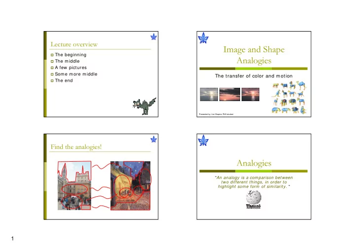
Image and Shape The beginning Analogies The middle A few pictures - PowerPoint PPT Presentation

Lecture overview Image and Shape � The beginning Analogies � The middle � A few pictures � Some more middle The transfer of color and motion � The end Presented by: Lior Shapira, PhD student Find the analogies! Analogies “ An analogy is a comparison between two different things, in order to highlight some form of similarity. “ 1

Find the analogies! Find the analogies! Find the analogies! Find the analogies! 2

Find the analogies! Find the analogies! What ’ s our purpose? � Transfer the colors of one image to Image Color Transfer another � Analyze images � Find correspondence (which color goes where?) � Perform a smooth transfer of the colors 3

The RGB Domain Finding a model for the data � A regular image � Working in geometric coordinates The RGB Domain The RGB Domain � Image pixels in RGB space � Image pixels in RGB space 4

K-means Clustering � To find analogies we ’ ll attempt to find � A very simple way to cluster data correspondences between clusters in the data � ( � ) 5 n 2 ∑ ∑ − arg min m x C � i j , i j � Clustering of data is a method by which { } = = C , m j 1 i 1 j i j , large sets of data is grouped together into � clusters of smaller sets of similar data ⎧ ∈ 1 x the j-th cluster = ⎨ i � m i j , ∉ ⎩ 0 x the j-th cluster i 5 ∑ = m 1 i j , = j 1 � → ∈ any x a single cluster i K-means for Clustering K-means for Clustering � K-means � K-means � Start with a random � Start with a random guess of cluster guess of cluster centers centers � Determine the � Determine the membership of each membership of each data points data points � Adjust the cluster � Adjust the cluster centers centers 5

K-means K-means for Clustering 1. Ask user how many clusters they ’ d like. � K-means (e.g. k= 5) � Start with a random guess of cluster centers � Determine the membership of each data points � Adjust the cluster centers K-means K-means Ask user how many Ask user how many 1. 1. clusters they ’ d like. clusters they ’ d like. (e.g. k= 5) (e.g. k= 5) Randomly guess k Randomly guess k 2. 2. cluster Center cluster Center locations locations Each datapoint finds 3. out which Center it ’ s closest to. (Thus each Center “ owns ” a set of datapoints) 6

K-means K-means Ask user how many Ask user how many 1. 1. clusters they ’ d like. clusters they ’ d like. (e.g. k= 5) (e.g. k= 5) Randomly guess k Randomly guess k 2. 2. cluster Center cluster Center locations locations Each datapoint finds Each datapoint finds 3. 3. out which Center it ’ s out which Center it ’ s closest to. closest to. Each Center finds the Each Center finds the 4. 4. centroid of the points centroid of the points it owns it owns Gaussians Limitations of K-means � Normal distribution (1D) � User inputs number of clusters ⎛ ( ) ⎞ � Sensitive to initial guesses − µ 2 1 x µ σ = ⎜ − ⎟ f x ( , ) exp ⎜ ⎟ � Converges to local minimum σ σ π 2 2 2 ⎝ ⎠ � Problematic with clusters of � Differing sizes � Differing densities � Non globular shapes � Difficulty with outliers 7

Gaussians Gaussians ( ) ( ) ⎛ ⎞ − − µ T Σ − µ 1 � 2D Gaussians x x 1 µ Σ = ⎜ − ⎟ f x ( , ) exp ⎜ ⎟ ( ) � d = 2 2 π d Σ ⎝ ⎠ 2 det( ) � x = random data point (2D vector) µ � = mean value (2D vector) Σ � = covariance matrix (2D matrix) Σ ⎛ ( ) ( ) ⎞ − µ T Σ − − µ 1 x x 1 µ Σ = ⎜ − ⎟ f x ( , ) exp ⎜ ⎟ ( ) π d Σ 2 ⎝ ⎠ 2 det( ) µ � The same equation holds for a 3D Gaussian Covariance Matrix Geometry Exploring Covariance Matrix = x random vector w h ( , ) i i i Σ = T V * D V * Σ ⎛ ⎞ σ 2 N cov( , ) w h 1 ∑ ( )( ) Σ = − µ − µ T = ⎜ = λ w ⎟ x x a v 1* σ i i 1 2 N ⎝ ⎠ cov( , ) h w = i 1 h = λ b v 2* Σ 2 is symmetric � ⇒ Σ Σ = T has eigendecomposition (svd) V * D V * � λ ≥ λ ≥ ≥ λ ... b � 1 2 d a Σ 8

GMMs – Gaussian Mixture Model 3D Gaussians � Suppose we have 1000 data points in 2D space (w,h) = x ( , , ) r g b i ⎛ σ ⎞ 2 W cov( , ) g r cov( , ) b r ⎜ r ⎟ N 1 ∑ ( )( ) Σ = − µ − µ T = ⎜ σ 2 x x cov( , ) r g cov( , ) b g ⎟ i i g N ⎜ ⎟ = σ i 1 2 cov( , ) r b cov( , ) g b ⎝ ⎠ b H The GMM assumption GMMs – Gaussian Mixture Model � Assume each data point is normally distributed � There are K components (Gaussians) � Obviously, there are 5 sets of underlying gaussians � Each k is specified with three parameters: W weight, mean, covariance matrix � The total density function is: ( ) ( ) ⎛ ⎞ T − − µ Σ − µ 1 x x K ∑ 1 ⎜ ⎟ Θ = α − j j j f x ( ) exp ⎜ ⎟ j ( ) 2 π d Σ = 2 det( ) j 1 ⎝ ⎠ j Θ = α µ Σ K { , , } = j j j j 1 K ∑ α = α ≥ ∀ α = weight 0 j 1 j j = j 1 H 9

EM Basics The EM algorithm (Dempster, Laird and Rubin, 1977) � Objective: µ Σ Θ Given N data points, find maximum likelihood estimation of : i i Θ = Θ arg max f x ( ,..., x ) 1 N Θ � Algorithm: Θ 1. Guess initial 2. Perform E step (expectation) Θ � Based on , associate each data point with specific gaussian 3. Perform M step (maximization) Θ � Based on data points clustering, maximize 4. Repeat 2-3 until convergence (~ tens iterations) Raw data GMMs (K = 6) Total Density Function EM Example EM Details � E-Step (estimate probability that point t associated to gaussian j) : α µ Σ data point t f x ( , ) = j t j j = = w j 1,..., K t 1,..., N ∑ t j , K α µ Σ blue: w t,j f x ( , ) = i t i i i 1 M-Step (estimate new parameters) : � N 1 ∑ α = new w j t j , N = t 1 Gaussian j ∑ N w x µ = = new t j , t t 1 ∑ j N w = t j , t 1 ∑ N − µ − µ new new T w ( x )( x ) Σ = = t j , t j t j new t 1 ∑ j N w = t j , t 1 10

EM Example EM Example EM Example EM Example 11

EM Example EM Example Applying EM on RGB space EM Example � Suppose we cluster the points for 2 clusters 12

Pixel Clusters Back to Clustering � The result in image space � We want to label “ close ” pixels with the same label � Proposed metric: label pixels from the same gaussian with same label � Label according to max probability: = label t ( ) arg max( w ) t j , j � Number of labels = K Graph-Cut optimization Formalizing a New Labeling Problem � Previous model for labeling: � A Problem: Noise = j 1,..., K gaussians ( ) = = f label p ( ) arg max( w ) ∈Ρ p p j , p ( image pixels ) j � A new model for labeling. Minimize E: = + λ E f ( ) E ( ) f E ( ) f data smooth � f = Labeling function, assigns label f p for each pixel p � Why? Pixel labeling is done independently for each pixel, � E data = Data Term ignoring the spatial relationships between pixels! � E smooth = Smooth Term � Lamda is a free parameter 13

Minimizing the Energy The Energy Function = + λ E f ( ) E ( ) f E ( ) f data smooth � Labels Set: { j= 1, … ,K } � Solving Min(E) is NP-hard � It is possible to approximate the solution using � E data : iterative methods � Penalize disagreement between pixel and the GMM ∑ = − � Graph-Cuts based methods approximate the D ( f ) D ( f ) 1 w p p p p p f , p global solution (up to constant factor) in ∈ p Pixels polynomial time � E smooth : � Penalize disagreement between two pixels, unless it ’ s a natural edge in the image = ⎧ 0 f f ∑ = ⎨ − p q V ( f , f ) V ( f , f ) p q , p q p q , p q ⎩ 1 dist p q ( , ) ow p q , neighbors � dist(p,q) = normalized color-distance between p,q Algorithm for Minimizing E(f) α -expansion moves � When using iterative methods, each iteration some of the 1. Start with an arbitrary labeling pixels change their labeling 2. Set success = 0 3. For each label j 3.1 Find f ’ = argmin(E(f ’ )) among f ’ within one α -expansion of f 3.2 If E(f ’ ) < E(f), set f = f ’ and success = 1 4. If (success = = 1) Goto 2 5. Return f Current One Pixel α - β -swap α -expansion Labeling Move Move Move � Given a label α , a move from partition P (labeling f) to a new partition P ’ (labeling f ’ ) is called an α -expansion move How to find argmin(E(f’)) ? if: ⊂ ∧ ⊂ ∀ ≠ α P P ' P ' P l α α l l 14