Hubble Catalog of variables - Presentation @Napoli Observatory - PDF document
See discussions, stats, and author profiles for this publication at: https://www.researchgate.net/publication/309634589 Hubble Catalog of variables - Presentation @Napoli Observatory Presentation October 2016 CITATIONS READS 0 17 1 author:
See discussions, stats, and author profiles for this publication at: https://www.researchgate.net/publication/309634589 Hubble Catalog of variables - Presentation @Napoli Observatory Presentation · October 2016 CITATIONS READS 0 17 1 author: Panagiotis Gavras RHEA Group for ESA 53 PUBLICATIONS 2,918 CITATIONS SEE PROFILE Some of the authors of this publication are also working on these related projects: The CPMDS catalogue of common proper motion double stars in the Bordeaux Carte du Ciel zone View project Gaia Mission View project All content following this page was uploaded by Panagiotis Gavras on 03 November 2016. The user has requested enhancement of the downloaded file.
Hubble Catalog of Variables Panagiotis Gavras on behalf of the HCV team Napoli , 19 Oct 2016
Outline • The HCV project • Hubble Source Catalog • Variability detection • Pipeline • First Results
Hubble Catalog of Variables • 3-Year ESA funded project (2015-2018) • Goal of the project is to develop a set of algorithms which will identify candidate variables among the sources included in Hubble Source Catalog (HSC). • At the end of the project we will produce the first version of Hubble Catalog of Variables (HCV). This catalog will be ingested to MAST portal and ESA Science Archives. • Finally the pipeline will be deployed in STScI and run regularly in order to produce updated versions of HCV.
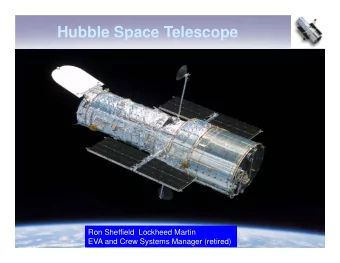
Hubble Source Catalog • Hubble Source Catalog (Whitmore et al., 2016) is a catalog with the majority of all objects ever observed by Hubble Space Telescope (HST). • It is developed and maintained by the Space Telescope Science Institute (STScI). • The HSC is designed to optimise science from the Hubble Space Telescope by combining the tens of thousands of visit-based source lists in the Hubble Legacy Archive (HLA) into a single master catalog.
HSC : What’s inside • HSC v2.0 released 29 Sep 2016. • 90 million sources and 383 million detections. • Photometry from WFPC2, ACS/WFC, WFC3/UVIS, and WFC3/IR. • In total there are 112 filter/detector combinations.
HSC : What’s inside • The mean photometric accuracy is better than 0.10 mag (may go down to 0.02mag). • The absolute astrometric accuracy is better than 0.1 arcsec. • 91% of HSC has coverage from Pan-STARRS, SDSS, or 2MASS.
HSC: Things one should know • Coverage can be very non-uniform (unlike surveys such as SDSS). • Current WFPC2, ACS/WFC and WFC3 source lists are of variable quality. • The default is to show all HSC objects. This may include a large number of artifacts . Requesting Numimages > 1 (or more) should filter out many artifacts. • Doubling: There are occasionally cases where not all the detections of the same source are matched together into a single objects. • Bad Images : Images taken when Hubble has lost lock on guide stars (generally after an earth occultation) are the primary cause of bad images.
HSC: Access • MAST Discovery portal: https://mast.stsci.edu/portal/Mashup/Clients/Mast/Portal.html • Online form : https://archive.stsci.edu/hst/hsc_sum/search.php • CasJobs : http://mastweb.stsci.edu/hcasjobs/home.aspx
Variability
Variability detection methods • Direct image comparison (transient detection) SN1987a Before After
Variability detection methods • Direct image comparison (transient detection) • Periodicity search
Variability detection methods • Direct image comparison (transient detection) • Periodicity search • Lightcurve analysis using variability indexes
Variability Indexes (VI) • They are numerical parameters characterizing the degree of variability of an object. • Different VIs are sensitive to different type of variability. • One expect a variable to have a significant different value in some VI than non-variables. • 2 Types of Variability Indexes • Scatter-based • Correlation-based
Scatter-based Variability Indexes • reduced χ 2 test • Standard deviation σ • MAD • Interquartile range (IQR) N | m i − median( m i ) | � RoMS = ( N − 1) − 1 . σ i • Robust Median Statistics (RoMS) i = 1 N 1 For a non-variable object, the expected value � σ 2 m ) 2 − σ 2 [( m i − ¯ i ] . NXS = m 2 N ¯ • Normalised Excess Variance σ 2NXS i = 1 v = ( m i − σ i ) max − ( m i + σ i ) min Here we use the symbol for the n ( m i − σ i ) max + ( m i + σ i ) min • Peak-to-Peak variability v where ( m ) and ( m ) See more at Sokolovsky et al, 2016
Correlation-based Variability Indexes measurements obtained in two filters b � n � b i − ¯ � � v i − ¯ � 1 b v � I = • Welch-Stetson I n ( n − 1) σ b i σ v i i = 1 where b ( v ) are the measured magnit n k = 1 w k sgn( P k ) √ | P k | � • Stetson’s indexes J,K,L J = n � k = 1 w k • and variations… time weighted, togram: where sgn is the sign fu N � � � v i − ¯ v � n v � magnitude limited 1 / N � � � n v − 1 � � σ vi i = 1 � � K = . � � 2 N � � v i − ¯ v n v 1 / N � • Consecutive same-sign deviations from n v − 1 σ vi i = 1 mean magnitude (CSSD) For a Gaussian magnitude dist � � L = π / 2 JK ( w / w all ) ( where ( w w ) is the ratio See more at Sokolovsky et al, 2016
Correlation-based Variability Indexes The index E x is computed according to the equation: � � N scan − 1 N scan � median i − median j • Excursions, E x 2 � � � � � E x = N scan ( N scan − 1) � σ 2 i + σ 2 i = 1 j > i , j where N is the number of scans, N ( N 1) 2 N − 1 i = 1 ( m i + 1 − m i ) 2 / ( N − 1) � • Von Neumann ratio, η η = δ 2 . σ 2 = N m ) 2 / ( N − 1) i = 1 ( m i − ¯ � Abbe value • Excess Abbe value Ε Α E A ≡ A sub − A where is the m tection statistic is defined as � 1 � r i , 1 M � 2 + ... + r i , k i � + r i , 2 • S B variability detection statistics � S B = NM σ i , 1 σ i , 2 σ i , k i i = 1 where N represents the total number of data p See more at Sokolovsky et al, 2016
Ο k but how do you define which source is variable? • We have more than 90 million sources divided in Groups (targets). • Less than 10% of the sources are variable. • General Idea : We have a sea of constant sources and few variables that should stand out in some variability indexes.
Ο k but how do you define which source is variable?
Ο k but how do you define which source is variable?
Ο k but how do you define which source is variable?
Ο k but how do you define which source is variable?
Ο k but how do you define which source is variable?
How does a source behave in different VIs?
How does a source behave in different VIs? Remember : Different VIs are sensitive to different type of variability
How does a source behave in different VIs? …. and different filters
Selection of Candidates (1st method)
Selection of Candidates (1st method)
Selection of Candidates (1st method)
Selection of Candidates (1st method)
Selection of Candidates (1st method)
VI Performance • Using this selection method we evaluated the performance of each variability index (2014), we compute the completeness C and pu Number of selected variables C = • Completeness Total number of confirmed variables • Purity Number of selected variables P = Total number of selected candidates • F-Score as well as the fidelity F -score 11 which is the har F 1 = 2( C × P ) / ( C + P ) . F reaches a maximum o
VI Performance C(F max )=0.706 P(F max )=0.740 F max =0.723 at 10.8 σ C(F max )=0.569 P(F max )=0.899 F max =0.697 at 6.0 σ C(F max )=0.821 P(F max )=0.825 F max =0.823 at 16.6 σ 1 1 1 C C C 0.9 0.9 0.9 P P P 0.8 F 0.8 F F 0.8 0.7 0.7 0.7 0.6 0.6 0.6 0.5 0.5 0.5 0.4 0.4 0.4 0.3 0.3 0.3 0.2 0.2 0.2 0.1 0.1 0.1 0 0 0 5 10 15 20 25 30 35 40 45 50 0 5 10 15 20 25 30 35 40 45 50 0 χ 2 0 5 10 15 20 25 30 35 40 45 50 σ w cut-off in σ red cut-off in σ 1/ η cut-off in σ
VI Performance 0.5 0.45 0.4 0.35 0.3 F 1 max 0.25 0.2 0.15 0.1 σ IQR 0.05 1/ η 0 0 50 100 150 200 250 300 N
Selection of Candidates (2nd method) • Principal Component Analysis (PCA) on the normalized variability indexes • Principal component analysis (Pearson 1901) linearly and orthogonally transforms a dataset onto a new set of un-correlated axes (the eigenvectors of the variance-covariance matrix of the data), where the data variance is being high-lighted. • These eigenvectors are called the principal components (PCs). Each observation x j of the original data, composed of m variables, is expressed as m � x j = a j,i · PCi i =1 where a i is the admixture coefficient of the principal component PCi. The coefficients a i are the data coordinates in the new axes. There exist a maximum of m PCs.
PCA on the normalized indexes F606W F814W Scree plot representing the variances for the PC1 & PC2 for the M31 Halo11 PCA implementation in 15 most significant Principal Components as two filters. applied in the M31 Halo11 field. Moretti et al., in prep
Selection of Candidates (2nd method) LPV/Semiregulars RR Lyrae RR Lyrae candidates Eclipsing binaries Dwarf Cepheids Anomalous Cepheids * Post-AGB stars Moretti et al., in prep
Recommend
More recommend
Explore More Topics
Stay informed with curated content and fresh updates.

