http://vision.unipv.it/ PROTEIN STRUCTURE ANALYSIS THROUGH HOUGH - PowerPoint PPT Presentation
http://vision.unipv.it/ PROTEIN STRUCTURE ANALYSIS THROUGH HOUGH TRANSFORM AND RANGE TREE VIRGINIO CANTONI, Dipartimento di Informatica e Sistemistica, Universit di PAVIA, virginio.cantoni@unipv.it ELIO MATTIA, Center for Systems Chemistry,
http://vision.unipv.it/ PROTEIN STRUCTURE ANALYSIS THROUGH HOUGH TRANSFORM AND RANGE TREE VIRGINIO CANTONI, Dipartimento di Informatica e Sistemistica, Università di PAVIA, virginio.cantoni@unipv.it ELIO MATTIA, Center for Systems Chemistry, Rijksuniversiteit Groningen, Groningen, The Netherlands, E.Mattia@rug.nl
Overview • Searching in a database of protein structures – Pairwise comparison – All-to-All comparison – Search for a structural “motif” 2
General Hough transform approach to protein structure comparison 3C Vision c ues, c ontexts and c hannels Elsevier (April 2011) V. Cantoni, S. Levialdi, B. Zavidovique Università di Pavia, Roma, Université de Paris XI
Paul Hough , 1959 : straight lines y = mx+q q = y i -mx i q y x m Image plane Parameter space - < m, q < + r = x cos( q ) + y sin( q ) 0 < r < L 2; - q 4
Example 5
Richard Duda and Peter Hart 1972: Circles f((x,y),x c ,y c ,r) = (y-y c ) 2 +(x-x c ) 2 -r 2 =0 y y c x x c Image plane Parameter spaces y o dy i /dx i (x c ,y c ) 6 Parameter space x y c = -1/m i x c + (y i - m i x i ) o
Exemple de vote: cercle 7
Dana H. Ballard 1981: Generalized HT Mapping rule X 0 = x + r cos( a ) ; Y 0 = y + r sin( a ) 8
Exemple de vote : clé 1 9
Basics on Proteins • A protein is an ordered sequence of amino acids • Building blocks: 20 amino acid residues. • Three- dimensional shapes (“fold”) vary enormously. 10
Levels of protein structure representation Primary structure Secondary structure Tertiary structure Quaternary structure 11
Primary structure: the sequence of amino acids 12
Secondary structures Three basic components: • helix • sheet • Loops (linear connections between the components) 13
The helix • One of the most closely packed arrangement of residues. • ~40% of residues in globular proteins 14
The sheet loosely packed Parallel Antiparallel Twisted arrangement of residues. 15
Secondary Structures Representation • Secondary structures are represented as linear vectors (segments): the axis for the alpha helix and the best fit segment for a strand • An alignment algorithm is used to match an helix segments with known axes to determine helix axis. Direct segment fits are made to fit sheet strands. 16
Secondary Structure Determination • Programs: DSSP and STRIDE. • On the average 4.8% of the target residues were differently assigned, this number reaching 12% for certain targets. 17
Distribution of segment lenght 18
Protein Structure Comparison Given a What are motif or the most PDB domain or similar protein folds ? 19
Secondary structure representation • Each segment is associated to a secondary structure and is displayed as a cylinder • The protein is represented by and ordered sequence of cylinder with two labels: helices or strands 20
GHT applied to proteins • For every protein, the distance ( r ) of every secondary structure from a reference point (RP, eg the geometric center of the protein) and the angle (theta) between the direction of the secondary structure in the 3D space and the segment linking the center of that secondary structure with the RP are first calculated. (GH reference table RT) 21
In the way of GHT (simplified 2D representation) helices and strands Query protein (scaled 0.5) Mapping Rule Votes Space 22
In the way of GHT helices and strands Query protein Mapping Rule Votes Space 23
Proteins: the 3D solution 24
GH parameters spaces Credits: Elio Mattia 25
GHT applied to proteins • In the 3D space of a given “object protein”, every secondary structure of a “model protein” votes a circumference of points starting from every secondary structure of the object protein. • If the proteins are similar in shape, the circumferences will all intersect in a given point. 26
Main characteristics • the mapping rule, for each compatible correspondent, in 3D is a circle on a plane perpendicular to the axis of the secondary structure • Other information can be exploited to increase the S/N ratio: – the length of the secondary structure – the residues properties contained in the SS – any other (biochemical, morphological, etc.) peculiarities. 27
The implementation • The voting space is smoothed by accumulation of nearby votes (within a given radius) for each point • After smoothing, the highest peaks in the voting space are detected (avoiding to pick high votes that however are not the top of a peak but lie close to one such peak) • Only the relevant votes are stored in memory: there isn’t a matrix with all the possible cells. 28
Smoothing Algorithm • Smoothing is performed by accumulating votes within a given radius, for every point in the vote space. • The classic version, i.e., checking every vote for the vicinity condition, has been proven to be too time- consuming for applications, with a time complexity of O(n 2 ), where n is the number of votes in the vote space. • The smoothing problem can be seen as an “orthogonal search” problem, i.e., finding points within a given cube in space. • A particular structure has been implemented for solving this problem with a O(n log 3 (n)) complexity: Range Trees. 29
Ortogonal range tree X - range tree Y - range tree S , i S c h i I 30
Ortogonal range tree 31
The implementation • The comparison of ONE (1) object protein with MANY (N) model proteins is accomplished by sorting the votes of the top peaks in the spaces of each of the (N) model proteins. • The sorting is carried out in TWO ways: either the smoothed votes themselves are sorted, or the differences between the two highest peaks in each of the (N) voting spaces are sorted. 32
First results 33
Testing on Motif Retrieval • The developed algorithm makes a new approach for protein structural comparison available. • The main application of this new approach is to classify protein structures and to retrieve structural motifs which are common of a given protein function. • Indeed, tests were performed on motif retrieval. • As an example, a motif (present in the Ubiquitin Conjugating Enzyme) was found in other proteins which are known to contain it. • Further testing will be done with the parallel implementation of the software. 34
Much experimentation allowed • Computationally, the results might vary substantially if any of the following parameters are varied: – The mesh of the voting space (in Ångström) – The mesh of the voting circumference (how many votes in each circumference) – The radius of smoothing – The radius of tolerance for avoiding “false peaks” when detecting peaks – The normalization factor (linear, square root, etc.) 35
Recommend
More recommend
Explore More Topics
Stay informed with curated content and fresh updates.
