How to use (can we use) the multiple linear regression method for a - PowerPoint PPT Presentation
How to use (can we use) the multiple linear regression method for a classification problem ? Ricco Rakotomalala Universit Lumire Lyon 2 Ricco Rakotomalala 1 Tanagra - http://data-mining-tutorials.blogspot.fr/ Ricco Rakotomalala 2
How to use (can we use) the multiple linear regression method for a classification problem ? Ricco Rakotomalala Université Lumière Lyon 2 Ricco Rakotomalala 1 Tanagra - http://data-mining-tutorials.blogspot.fr/
Ricco Rakotomalala 2 Tanagra - http://data-mining-tutorials.blogspot.fr/
Supervised learning : continuous vs. discrete target attribute Classification problem Regression analysis Y discrete target attribute Y continuous target attribute X descriptors, cont. or disc. X descriptors, continuous or discrete We want to construct a prediction function f(.) such as … Problems: Y choosing the function f(.) f ( X , ) estimating its parameters all the calculations are based on a sample Evaluating the quality of the predictions Quadratic error function Error rate Sum of squared error 0/1 loss (good or bad classification) 1 ˆ ˆ ET [ Y , f ( X , )] ˆ ˆ 2 S [ Y f ( X , )] card ( ) ˆ ˆ 1 si Y f ( X , ) où [.] ˆ ˆ 0 si Y f ( X , ) Ricco Rakotomalala 3 Tanagra - http://data-mining-tutorials.blogspot.fr/
Multiple linear regression: a reminder • Modeling with linear prediction function • Continuous dependent variable Z • Continuous (or dummy coded) explanatory variables, X 1 , X 2 , … z a a x a x a x ; i 1 , , n 0 1 , 1 2 , 2 , i i i p i p i The error term captures all the factors which influence the dependent variable other than the explanatory variables i.e. • le relationship between the dependent and the explanatory variables is not necessarily linear • some relevant variables are not included in the model • sampling fluctuation ˆ is the residual, this is the difference between the observed value of the dependent variable and its estimated value by the model is the parameter vector, we want to estimate its values on a ( a , a , , a ) sample 0 1 p Ricco Rakotomalala 4 Tanagra - http://data-mining-tutorials.blogspot.fr/
Linear regression of an indicator variable : the binary case -- Y {+, -} In the two classes problem 1 , if y i (Positive vs. Negative), we can code z i the target variable Y as follows 0 , if y i We observe that E ( Z ) P ( Y ) i i Thus… E ( Z ) P ( Y ) a a x a x i i 0 1 i , 1 p i , p Can we use the linear regression to estimate the posterior probability P(Y=+ / X) ??? >> the linear combination is defined between – and + , this is not a probability >> the assumptions under the OLS approach are violated Ricco Rakotomalala 5 Tanagra - http://data-mining-tutorials.blogspot.fr/
Simple linear regression: a geometrical point of view The linear combination cannot used to estimate the probability P(Y=+/X), … But it can be used to separate the groups !!! 1.4 E.g. Linear regression 1.2 + z a a x 1 i 0 1 i , 1 i 0 /1 ) 0.8 Z (endogène recodée en 0.6 0.4 - y = -0.9797x + 2.142 2 = 0.6858 R 0.2 0 0 0.5 1 1.5 2 2.5 3 -0.2 X (e xogè ne ) How to define this threshold ? Ricco Rakotomalala 6 Tanagra - http://data-mining-tutorials.blogspot.fr/
Decision rule with the 0/1 coding of the target attribute For a two classes problem, 1 , si y we can code the target i z i attribute as follows: 0 , si y i We perform the linear regression z a a x a x a x (OLS: ordinary least squares i 0 1 i , 1 2 i , 2 p i , p i method) We obtain the estimated ˆ ˆ ˆ ˆ ˆ z a a x a x a x coefficients i 0 1 i , 1 2 i , 2 p i , p ˆ , si z z ˆ i Decision rule y i ˆ , si z z i z P ( Y ) Mean of « z » i.e. Ricco Rakotomalala 7 Tanagra - http://data-mining-tutorials.blogspot.fr/
Decision rule with another coding scheme n , si y i We can use another n z i coding scheme n , si y i n Regression analysis z a a x a x a x i 0 1 i , 1 2 i , 2 p i , p i ˆ ˆ ˆ ˆ ˆ OLS estimators z a a x a x a x i 0 1 i , 1 2 i , 2 p i , p ˆ , si z 0 ˆ i y Decision rule ˆ i , si z 0 We observe that… i 1 n n z n n ( ) n n n 0 Ricco Rakotomalala 8 Tanagra - http://data-mining-tutorials.blogspot.fr/
Ricco Rakotomalala 9 Tanagra - http://data-mining-tutorials.blogspot.fr/
Linear classifier: a straight line to separate the groups n = 100 instances p = 2 predictive variables K = 2 groups with (n 1 = n 2 = 50) 3.0 2.5 The linear approaches virginica induces a linear 2.0 frontier to separate the groups. versicolor 1.5 1.0 0.5 2.0 3.0 4.0 5.0 6.0 7.0 8.0 Ricco Rakotomalala 10 Tanagra - http://data-mining-tutorials.blogspot.fr/
Equivalence between the results of regression and linear discriminant analysis Global results 0.7198 R² Regression Adjusted-R 0.713979 Sigma error 0.268752 124.5641 F-Test (2,97) (0.000000) Coefficients Attribute Coef. std t(97) p-value -0.198 -3.428 pet.length 0.057648 0.000893 -0.663 -5.921 pet.width 0.112044 0.000000 2.082 12.326 Intercept 0.168871 0.000000 MANOVA Discriminant analysis 2 1 R 1 0 . 7198 0 . 2802 Stat Value p-value Wilks' Lambda 0.2802 - Bartlett -- C(2) 123.3935 0 2 F t Rao -- F(2, 97) 124.5641 0 j j 2 11 . 754 ( 3 . 428 ) , LDA Summary Statistical Evaluation Classification functions Score function Wilks L. Partial L. F(1,97) p-value Attribute versicolor virginica D(X) 0.314202 0.89192 11.754 0.000893 -2.765 pet.length 14.40029 17.164859 0.381538 0.734509 35.061 0.000000 -9.280 pet.width 7.824622 17.104674 - 29.116 constant -36.55349 -65.66983 We know how to j j 2 . 765 0 . 198 13 . 988 calculate directly ! 9 . 280 0 . 663 13 . 988 Ricco Rakotomalala 11 29 . 116 2 . 082 13 . 988 Tanagra - http://data-mining-tutorials.blogspot.fr/
When the classes are not balanced (n 1 n 2 ) n = 183 with n 1 = 96, n 2 = 87 Global results R² 0.2753 Regression Adjusted-R 0.2672 Sigma error 0.4287 F-Test (2,180) 34.1851 Coefficients Attribute Coef. std t(180) p-value max.rate -0.0076 0.0014 -5.3940 0.0000 oldpeak 0.1701 0.0327 5.1990 0.0000 Intercept 0.8463 0.2200 3.8461 0.0002 MANOVA Discriminant analysis 2 1 R 1 0 . 2753 0 . 7247 Stat Value p-value Wilks' Lambda 0.7247 - Bartlett -- C(2) 57.9534 0 Rao -- F(2, 180) 34.1851 0 (-5.3940)² = 29.0951 (5.1990)² = 27.0301 LDA Summary Classification functions Statistical Evaluation Fonction Attribute present absent Wilks L. Partial L. F(1,180) p-value score max.rate 0.3113 0.3530 -0.0417 0.8419 0.8609 29.0951 0.0000 oldpeak 2.3975 1.4665 0.9310 0.8336 0.8694 27.0301 0.0000 constant -23.9246 -28.6913 4.7667 - The intercepts are -0.0417 / -0.0076 = 5.4721 different . The decision rules 0.9310 / 0.1701 = 5.4721 are different !!! 4.7667 / 0.8463 = 5.6323 Ricco Rakotomalala 12 Tanagra - http://data-mining-tutorials.blogspot.fr/
The induced frontiers when the classes are not balanced Linear regression Discriminant analysis (1) The intercepts are different (2) We have parallel lines to separate the groups (3) The model performances are different i.e. the confusion matrices are different (4) The magnitude of the gap depends on the degree of class imbalance Ricco Rakotomalala 13 Tanagra - http://data-mining-tutorials.blogspot.fr/
Regression vs. Linear discriminant analysis - Equivalence We can obtain the coefficients of the linear discriminant function from the results of the linear regression >> the models are exactly the same for balanced data >> the intercepts are different when n 1 n 2 , an additional correction is needed Warning, the statistical assumptions under the methods are not identical: • X are treated as fixed values in regression • the error term is particular to the regression • etc. Nevertheless, we can use the test for global significance of the model and the significance tests for coefficients, whatever the class distribution (balanced or imbalanced case). Ricco Rakotomalala 14 Tanagra - http://data-mining-tutorials.blogspot.fr/
Ricco Rakotomalala 15 Tanagra - http://data-mining-tutorials.blogspot.fr/
Recommend
More recommend
Explore More Topics
Stay informed with curated content and fresh updates.
