Hierarchical Modeling for Large Univariate Areal Data Abhi Datta 1 , - PowerPoint PPT Presentation
Hierarchical Modeling for Large Univariate Areal Data Abhi Datta 1 , Sudipto Banerjee 2 and Andrew O. Finley 3 July 31, 2017 1 Department of Biostatistics, Bloomberg School of Public Health, Johns Hopkins University, Baltimore, Maryland. 2
Hierarchical Modeling for Large Univariate Areal Data Abhi Datta 1 , Sudipto Banerjee 2 and Andrew O. Finley 3 July 31, 2017 1 Department of Biostatistics, Bloomberg School of Public Health, Johns Hopkins University, Baltimore, Maryland. 2 Department of Biostatistics, Fielding School of Public Health, University of California, Los Angeles. 3 Departments of Forestry and Geography, Michigan State University, East Lansing, Michigan.
Areal data Figure: Standardized stomach cancer incidence in 194 municipalities in Slovenia • Each datapoint is associated with a region like state, county, municipality etc. • Usually a result of aggregating point level data 1
Spatial disease mapping Standardized cancer incidence Socio-economic score Figure: Slovenia stomach cancer data • Goal: Identify factors (covariates) associated with the disease • Goal: Identify spatial pattern, if any, and smooth spatially • Inference is often restricted only to the given set of regions 2
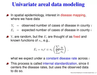
GLM for Spatial disease mapping • At unit (region) i , we observe response y i and covariate x i • g ( E ( y i )) = x ′ i β + w i where g ( · ) denotes a suitable link function Hierarchical areal model: k p 1 ( y i | x ′ i β + w i ) × N − 1 ( w | 0 , τ w Q ( ρ )) × p 2 ( β, τ w , ρ ) � i =1 • Notation: N − 1 ( m , Q ) denotes normal distribution with mean m and precision (inverse covariance) Q • p 1 denotes the functional form of the density corresponding to the link g ( · ) 3
How to model Q ( ρ ) • Choice of Q ( ρ ) should enable spatial smoothing • One possibility: Represent each region by a single point and use Gaussian Process covariance i.e. Q ( ρ ) − 1 = C ( m ( i ) , m ( j )) ij • Many possible choices to map the region i into a Euclidean coordinate m ( i ) • Is it appropriate to represent a large area with a single point? • Also GP approach is computationally very expensive • Alternate approach: Represent spatial information in terms of a graph depicting the relative orientation of the regions 4
CAR models • Conditional autoregressive (CAR) model (Besag, 1974; Clayton and Bernardinelli, 1992) • Areal data modeled as a graph or network: V is the set of vertices (regions) • i ∼ j if regions i and j share a common border • Adjacency matrix A = ( a ij ) such that a ij = I ( i ∼ j ) • n i is the number of neighbors of i • CAR model: w i | w − i ∼ N − 1 ( ρ � w j , τ w n i ) n i j | i ∼ j 5
CAR models • CAR model: w i | w − i ∼ N − 1 ( 1 � w j , τ w n i ) n i j | i ∼ j • w = ( w 1 , w 2 , . . . , w k ) ′ ∼ N − 1 (0 , τ w ( D − ρ A )) where D = diag ( n 1 , n 2 , . . . , n k ) • ρ = 1 ⇒ Improper distribution as ( D − A )1 = 0 (ICAR) • Can be still used as a prior for random effects • Cannot be used directly as a data generating model 6
CAR models • CAR model: w i | w − i ∼ N − 1 ( 1 � w j , τ w n i ) n i j | i ∼ j • w = ( w 1 , w 2 , . . . , w k ) ′ ∼ N − 1 (0 , τ w ( D − ρ A )) where D = diag ( n 1 , n 2 , . . . , n k ) • ρ = 1 ⇒ Improper distribution as ( D − A )1 = 0 (ICAR) • Can be still used as a prior for random effects • Cannot be used directly as a data generating model • ρ < 1 ⇒ Proper distribution with added parameter flexibility 6
SAR models • Simultaneous Autoregressive (SAR) model (Whittle, 1954) • Instead of taking the conditional route, SAR model proceeds by simultaneously modeling the random effects � w i = ρ b ij w j + ǫ i for i = 1 , 2 , . . . , k i � = j ind ∼ N − 1 (0 , τ i ) are errors independent of w • ǫ i • A common choice is to define b ij = I ( i ∼ j ) / n i • Joint distribution: w ∼ N − 1 (0 , ( I − ρ B ) ′ F ( I − ρ B )), B = ( b ij ) and F = diag ( τ 1 , τ 2 , . . . , τ k ) • ρ = 1 ⇒ Improper distribution 7
Interpretation of ρ in proper CAR and SAR models • Calibration of ρ as a correlation, e.g., (as reported in Banerjee et al. 2014) ρ = 0 . 80 yields 0 . 1 ≤ Moran’s I ≤ 0 . 15 , ρ = 0 . 90 yields 0 . 2 ≤ Moran’s I ≤ 0 . 25 , ρ = 0 . 99 yields Moran’s I ≤ 0 . 5 • So, used with random effects, scope of spatial pattern may be limited 8
Interpretation of ρ in proper CAR and SAR models • ρ cannot be interpreted as correlation between neighboring w i ’s (Wall, 2004; Assuncao and Krainski, 2009) Figure: Neighbor pair correlations as a function of ρ for proper CAR and SAR models over the graph of US states 8
SAR model and Cholesky factors • General SAR model: � w i = b ij w j + ǫ i for i = 1 , 2 , . . . , k i � = j • w ∼ N − 1 (0 , ( I − B ) ′ F ( I − B )) where F = diag ( τ 1 , τ 2 , . . . , τ k ) • Only proper when I − B is invertible which is not guaranteed for arbitrary B • SAR is essentially modeling the precision matrix through the Cholesky factor I − B 9
SAR model and Cholesky factors • General SAR model: � w i = b ij w j + ǫ i for i = 1 , 2 , . . . , k i � = j • w ∼ N − 1 (0 , ( I − B ) ′ F ( I − B )) where F = diag ( τ 1 , τ 2 , . . . , τ k ) • Only proper when I − B is invertible which is not guaranteed for arbitrary B • SAR is essentially modeling the precision matrix through the Cholesky factor I − B • Cholesky factors are not unique • We can always choose a lower triangular Cholesky factor 9
New model w 1 = ǫ 1 w 2 = b 21 w 1 + ǫ 2 w 3 = b 31 w 1 + b 32 w 2 + ǫ 3 . . . w k = b k 1 w 1 + b k 1 w 2 + . . . + b k , k − 1 w k − 1 + ǫ k • B = ( b ij ) is now a strictly lower triangular matrix. 10
New model • Advantages of lower triangular B : • w ∼ N − 1 (0 , ( I − B ) ′ F ( I − B )) is a proper distribution for any choice of lower triangular B • det( L ′ FL ) = � n i =1 τ i where F = diag ( τ 1 , . . . , τ k ) and L = I − B 1 + � k • w ′ L ′ FLw = τ 1 w 2 { j < i } w j b ij ) 2 i =2 τ i ( w i − � • Likelihood N − 1 ( w | 0 , ( I − B ) ′ F ( I − B )) can be computed using O ( k + s ) flops where s denotes the sparsity (number of non-zero entries) of B . • Even if k is large, evaluation of likelihood is fast if each region only shares border with a few others 10
Choice of B and F • How to specify B and F ? • Sparsity of B is desirable • If data had replicates for each region, there is large literature on fully data driven estimation of sparse Cholesky factors (Wu and Pourahmadi, 2003; Huang et al., 2006; Rothman et al., 2008; Levina et al., 2008; Wagaman and Levina, 2009; Lam and Fan, 2009) • Unfortunately many areal datasets lack replication 11
Choice of B and F • How to specify B and F ? • Sparsity of B is desirable • Like in NNGP set b ij = 0 for j outside neighbor sets N ( i ) • Pros: For graphs neighbor sets are naturally chosen: N ( i ) = { j | j ∼ i , j < i } • Cons: There is no covariance function on arbitrary graphs from which we can obtain non-zero b ij ’s and F 12
Autoregressive models on trees • D = ( d ij ) is the shortest distance matrix on the graph • If the graph was a tree (no loops), then ρ D = ( ρ d ij is then a valid autoregressive correlation matrix (AR(1) model on a tree, Basseville et al., 2006). • Areal graphs are loopy and are not usually trees 13
Local embedded spanning trees • Embedded spanning trees (EST) of a graph G is a subgraph of G which is a tree and spans all the vertices of G • Note that to specify w i = � j ∈ N ( i ) b ij w j + ǫ i we only need a joint distribution on { i } ∪ N ( i ) • Let G i denote the subgraph of G which includes vertices { i } ∪ N ( i ) and the edges among them • The subgraph T i of G i which only contains the edges { i ∼ j | j ∈ N ( i ) } is an embedded spanning tree of G i • Use the local embedded spanning trees T i to specify the b ij ’s and τ i 14
Directed acyclic graph autoregressive (DAGAR) model • AR i denotes the AR (1) distribution on T i • Solve for b ij and τ i such that E AR i ( w i | w N ( i ) ) = � j ∈ N ( i ) b ij w j and τ i = 1 / Var AR i ( w i | w N ( i ) ) • No edge is left out ! Figure: Decomposing a graph into a sequence of embedded spanning trees 15
Properties of DAGAR models • b ij = b i = ρ/ (1 + ( | N ( i ) | − 1) ρ 2 ) • τ i = (1 + ( | N ( i ) | − 1) ρ 2 ) / (1 − ρ 2 ) • det( Q DAGAR ) = � k i =1 τ i • Positive definite for any 0 ≤ ρ ≤ 1 • Interpretability of ρ : • If the graph is a tree, then DAGAR model is same as the AR(1) model on the tree i.e. correlation between d th order neighbors is ρ d for d = 1 , 2 , . . . • If the graph is a closed two-dimensional grid, then each neighbor pair correlation is ρ • p DAGAR ( w ) can be stored and evaluated using O ( e + k ) flops where e is the total number of neighbor pairs 16
Dependence on ordering • DAGAR model depends on the ordering of the regions when decomposing into local trees • We can define a DAGAR model for every ordering • Spatial regions do not have natural ordering • How to choose the ordering? • Coordinate based orderings were used in Datta et al., 2016; Stein, 2004; Vecchia, 1988 • Model averaging over orderings ? Too many possibilities ( k !) 17
Order-free model • Let Q be the average over DAGAR precision matrices corresponding to all k ! possible orderings 18
Order-free model • Let Q be the average over DAGAR precision matrices corresponding to all k ! possible orderings • Q is is free of ordering and available in closed form • Q ( i , j ) is non-zero if and only if either i ∼ j or i ≈ j 18
Recommend
More recommend
Explore More Topics
Stay informed with curated content and fresh updates.
