Fusing point and areal level space-time data with application to wet - PowerPoint PPT Presentation

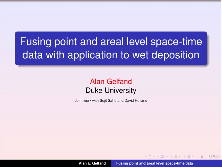
Fusing point and areal level space-time data with application to wet deposition Alan Gelfand Duke University Joint work with Sujit Sahu and David Holland Alan E. Gelfand Fusing point and areal level space-time data

Chemical Deposition Combustion of fossil fuel produces various chemicals including sulfate and nitrate gases. In the eastern U.S., most SO 2 , and NO x release attributed to power plants. Emitted to the air; wet deposition and dry deposition; interest in total deposition. Deposition means return to the earth’s surface by means of precipitation (rain or snow) for example. Wet Deposition = Precipitation × Concentration. Wet deposition is responsible for damage to lakes, forests, and streams. Alan E. Gelfand Fusing point and areal level space-time data

Chemical Deposition Combustion of fossil fuel produces various chemicals including sulfate and nitrate gases. In the eastern U.S., most SO 2 , and NO x release attributed to power plants. Emitted to the air; wet deposition and dry deposition; interest in total deposition. Deposition means return to the earth’s surface by means of precipitation (rain or snow) for example. Wet Deposition = Precipitation × Concentration. Wet deposition is responsible for damage to lakes, forests, and streams. Alan E. Gelfand Fusing point and areal level space-time data

Chemical Deposition Combustion of fossil fuel produces various chemicals including sulfate and nitrate gases. In the eastern U.S., most SO 2 , and NO x release attributed to power plants. Emitted to the air; wet deposition and dry deposition; interest in total deposition. Deposition means return to the earth’s surface by means of precipitation (rain or snow) for example. Wet Deposition = Precipitation × Concentration. Wet deposition is responsible for damage to lakes, forests, and streams. Alan E. Gelfand Fusing point and areal level space-time data

Chemical Deposition Combustion of fossil fuel produces various chemicals including sulfate and nitrate gases. In the eastern U.S., most SO 2 , and NO x release attributed to power plants. Emitted to the air; wet deposition and dry deposition; interest in total deposition. Deposition means return to the earth’s surface by means of precipitation (rain or snow) for example. Wet Deposition = Precipitation × Concentration. Wet deposition is responsible for damage to lakes, forests, and streams. Alan E. Gelfand Fusing point and areal level space-time data

Chemical Deposition Combustion of fossil fuel produces various chemicals including sulfate and nitrate gases. In the eastern U.S., most SO 2 , and NO x release attributed to power plants. Emitted to the air; wet deposition and dry deposition; interest in total deposition. Deposition means return to the earth’s surface by means of precipitation (rain or snow) for example. Wet Deposition = Precipitation × Concentration. Wet deposition is responsible for damage to lakes, forests, and streams. Alan E. Gelfand Fusing point and areal level space-time data

Chemical Deposition Combustion of fossil fuel produces various chemicals including sulfate and nitrate gases. In the eastern U.S., most SO 2 , and NO x release attributed to power plants. Emitted to the air; wet deposition and dry deposition; interest in total deposition. Deposition means return to the earth’s surface by means of precipitation (rain or snow) for example. Wet Deposition = Precipitation × Concentration. Wet deposition is responsible for damage to lakes, forests, and streams. Alan E. Gelfand Fusing point and areal level space-time data

The first stage likelihood f ( P , Z , Q | U , Y , X , V , ˜ V ) = f ( P | U , V ) × f ( Z | Y , V ) × f ( Q | X , ˜ V ) which takes the form �� n � � � T 1 exp ” 1 exp ” I ( v ( s i , t ) > 0 ) “ u ( s i , t ) “ y ( s i , t ) t = 1 i = 1 � �� � J ” I (˜ 1 exp v ( A j , t ) > 0 ) “ x ( A j , t ) j = 1 where 1 x denotes a degenerate distribution with point mass at x and I ( · ) is the indicator function. Alan E. Gelfand Fusing point and areal level space-time data

Deposition Model Y ( s i , t ) = β 0 + β 1 U ( s i , t ) + β 2 V ( s i , t ) + ( b 0 + b ( s i )) X ( A k i , t ) + η ( s i , t ) + ǫ ( s i , t ) . Spatially varying coefficients, b = ( b ( s 1 ) , . . ., b ( s n )) ′ is a Gaussian process (GP). Spatio-temporal intercept η t = ( η ( s 1 , t ) , . . ., η ( s n , t )) ′ is a GP independent in time. Allow for spatially varying calibration of CMAQ. Could imagine common η ( s i ) . ǫ ( s i , t ) ∼ N ( 0 , σ 2 ǫ ) , provides the nugget effect. Alan E. Gelfand Fusing point and areal level space-time data

The second stage models ... Precipitation U ( s i , t ) = α 0 + α 1 V ( s i , t ) + δ ( s i , t ) , where δ t = ( δ ( s 1 , t ) , . . ., δ ( s n , t )) ′ is a GP independent in time. CMAQ output X ( A j , t ) = γ 0 + γ 1 ˜ V ( A j , t ) + ψ ( A j , t ) , j = 1 , . . . , J . Assume ψ ( A j , t ) ∼ N ( 0 , σ 2 ψ ) , independently. Alan E. Gelfand Fusing point and areal level space-time data

Specification of latent processes Measurement Error Model (MEM) V ( s i , t ) ∼ N ( ˜ V ( A k i , t ) , σ 2 v ) , i = 1 , . . . , n , t = 1 , . . . , T . The process ˜ V ( A j , t ) is AR in time and CAR in space V ( A j , t ) = ρ ˜ ˜ V ( A j , t − 1 ) + ζ ( A j , t ) , � J � h ji ζ ( A i , t ) , σ 2 � ζ ζ ( A j , t ) ∼ N , m j i = 1 Let ∂ j define the m j neighboring grid cells of the cell A j . 1 � if i ∈ ∂ j m j h ji = 0 otherwise. Alan E. Gelfand Fusing point and areal level space-time data

AR in time and CAR in Space Assume the initial condition for ˜ V 0 : T V ( A j , 0 ) = 1 ˜ � X ( A j , t ) , T t = 1 giving ˜ V 0 . Now we can write the CAR in closed form: f (˜ V t | ˜ V t − 1 , ρ, σ 2 ζ ) ∝ � �� − 1 � ′ � � V t − ρ ˜ ˜ V t − ρ ˜ ˜ D − 1 ( I − H ) exp V t − 1 V t − 1 , 2 D is a diagonal matrix with entries σ 2 ζ / m j . Note that this is an improper CAR. Alan E. Gelfand Fusing point and areal level space-time data

National Atmospheric Deposition Program (NADP) NADP collects point-referenced data at several sites. They then use simple interpolation to produce maps. 6 6 8 5 9 9 6 6 11 12 7 4 4 4 13 7 6 6 7 15 6 11 5 6 15 6 6 12 10 8 8 14 19 11 16 6 8 16 17 16 14 20 13 16 12 19 13 12 18 18 18 16 22 15 12 16 17 19 20 20 16 19 13 30 15 28 24 18 14 11 11 10 22 13 17 10 16 13 11 11 13 19 22 8 13 9 17 14 18 10 12 8 10 21 21 15 16 16 14 15 10 11 11 15 13 14 16 13 11 17 13 13 15 16 8 9 4 14 10 12 10 10 16 12 12 13 20 11 Alan E. Gelfand Fusing point and areal level space-time data

The CMAQ model Community Multi-scale Air Quality Model (CMAQ) A computer simulation model which produces “averaged” output on 36km, 12 km(used here), and now 4 km grid cells Uses variables such as power station emission volumes, meteorological data, land-use, etc. with atmospheric science (appropriate differential equations) to predict deposition levels. Not driven by monitoring station data. Predictions are biased but no missing data; monitoring data provide more accurate deposition but “missingness” Alan E. Gelfand Fusing point and areal level space-time data

The CMAQ model Community Multi-scale Air Quality Model (CMAQ) A computer simulation model which produces “averaged” output on 36km, 12 km(used here), and now 4 km grid cells Uses variables such as power station emission volumes, meteorological data, land-use, etc. with atmospheric science (appropriate differential equations) to predict deposition levels. Not driven by monitoring station data. Predictions are biased but no missing data; monitoring data provide more accurate deposition but “missingness” Alan E. Gelfand Fusing point and areal level space-time data

The CMAQ model Community Multi-scale Air Quality Model (CMAQ) A computer simulation model which produces “averaged” output on 36km, 12 km(used here), and now 4 km grid cells Uses variables such as power station emission volumes, meteorological data, land-use, etc. with atmospheric science (appropriate differential equations) to predict deposition levels. Not driven by monitoring station data. Predictions are biased but no missing data; monitoring data provide more accurate deposition but “missingness” Alan E. Gelfand Fusing point and areal level space-time data

The CMAQ model Community Multi-scale Air Quality Model (CMAQ) A computer simulation model which produces “averaged” output on 36km, 12 km(used here), and now 4 km grid cells Uses variables such as power station emission volumes, meteorological data, land-use, etc. with atmospheric science (appropriate differential equations) to predict deposition levels. Not driven by monitoring station data. Predictions are biased but no missing data; monitoring data provide more accurate deposition but “missingness” Alan E. Gelfand Fusing point and areal level space-time data

Our Contribution A fully model-based framework for fusing the NADP and CMAQ wet deposition data To accommodate the point masses at 0, i.e., no wet deposition if no precipitation To accommodate misalignment between NADP data at points and CMAQ data at grid cells in a computational feasible way across space and time To provide spatial interpolation and temporal aggregation Both sulfate and nitrate deposition Alan E. Gelfand Fusing point and areal level space-time data