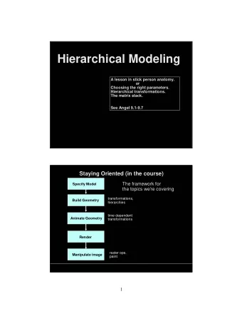
Hierarchical Modeling Hierarchical modeling has taken over the - - PowerPoint PPT Presentation

Hierarchical Modeling

Hierarchical modeling has taken over the landscape in contemporaery stochastic modeling Intent here is to show a range of examples In the development, we will also show the connections to Gibbs sampling, why Gibbs sampling and MCMC are ideally suited to fit these models We envision a three stage specification First stage: [data|model, parameters] Second stage: [model|parameters] Third stage: [(hyper)parameters]

Hierarchical Modeling – p. 1/13

Standard hierarchical linear model

First stage: Y|X, β ∼ N(Xβ, ΣY) Second stage: β|Z, α ∼ N(Zα, Σβ) Third stage: α ∼ N(α0, Σα) Assumes all Σ’s known. If not, inverse Gamma or Wishart priors Standard Gibbs loop to update; conjugacy for all full conditionals

Hierarchical Modeling – p. 2/13

CIHM

Conditionally independent hierarchical model

Πi[Yi|θi]Πi[θi|η][η]

Exchangeable θi Shrinkage - borrowing strength if η unknown Includes hierarchical GLM, i.e., nonGaussian first stage

Hierarchical Modeling – p. 3/13

Random effects

Random effects are usually assumed to be normally distributed with an associated variance component Typical linear version:

Yij = XT

ijβ + φi + ǫij

β has a Gaussian prior φi iid ∼ N(0, σ2

φ)

ǫij iid ∼ N(0, σ2

ǫ )

Priors on variance components, σ2

φ, σ2 ǫ (with care)

Again, can have a nonGaussian first stage

Hierarchical Modeling – p. 4/13

Missing data

Often have missing data Gibbs sampler (MCMC) extends the E-M algorithm to provide full posterior inference rather than an MLE with an asymptotic variance Simple example: Multivariate normal, Yi ∼ N(µ, Σ) Some components of some of the Yi are missing A usual Gibbs loop: update parameters given missing data, update missing data given parameters Simple example: Missing categorical counts with a multinomial model Some categories are aggregated/collapsed so counts for the disaggregated categories are missing Again, usual Gibbs loop: update parameters given all counts, update missing counts given parameters

Hierarchical Modeling – p. 5/13

Binary data models

Usual binary response model is logit or probit Illustrate for probit

Yi ∼ Bernoulli(p(Xi)) (can be Bi(ni, p(Xi))) Φ−1(p(Xi)) = Xiβ with a prior on β

Awkward to sample β in this form Introduce Zi ∼ N(Xiβ, 1)

P(Yi = 1) = Φ(Xiβ) = 1 − Φ(−Xiβ) = P(Zi ≥ 0)

So, Gibbs loop: update Z’s given β, y (truncated normal), update β given Z’s and y (usual normal updating) Can extend to ordinal categorical data; multiple unknown cut points

Hierarchical Modeling – p. 6/13

Growth Curves

Typically, individual level curves centered around a population level curve Need population level curves to see average behavior

• f process

Need individual level curves to prescribe individual level treatment Model: If Yij is jth measurement for ith individual,

Yij = g(Xij, Zi, βi) + ǫij ǫij ∼ N(0, σ2

i )

βi = β + ηi (or replace β with a regression in the Zi)

Hierarchical Modeling – p. 7/13

Mixture models

Y ∼ L

l=1 plfl(Y|θl), e.g., a normal mixture

Also called classification problem or discriminant analysis

L fixed or unknown?

Observe Yi, i = 1, 2, ..., n Label for Yi is not observed (latent) If Li = l, then Yi ∼ fl(Y|θl) So model is:

Πi[Yi|Li, θ][Πi[Li|α][α, θ]

Gibbs loop. Update β, α given L’s and data. Update L’s given β, α and data (discrete distribution) Covariates? In θl’s? In pl’s?

Hierarchical Modeling – p. 8/13

Errors in variables models

Seek the relationship between say Y and X Observe say W a surrogate for X, perhaps observe Z, a surrogate for Y Model W|X - measurement error model; model X|W - Berkson model Model in first case:

Πi[Zi|Yi, γ][Yi|Xi, β][Wi|Xi, γ][Xi|α]

Model in second case:

Πi[Zi|Yi, γ][Yi|Xi, β][Xi|Wi, γ]

Validation data: Perhaps some X, Y pairs; perhaps some X, W pairs

Hierarchical Modeling – p. 9/13

Change point models

Frequently, interest in a change in regime Need idea of a “least” significant change Two sampling scenarios - (i) full set of data. Try to find, retrospectively, if changes occurred and when, (ii) sequential data, try to identify changes as we collect. Simple first scenario example: f1(y|θ1) density before the change point; f2(y|θ2) density after the change point With data Yi, i = 1, 2, ..., n, then K, change point indicator, i.e., K = k means change at observation

k + 1; k = n means “no change.” Then, model is L(θ1, θ2, k; y) = Πk

i=1f1(yi|θ1)Πn i=k+1f2(yi|θ2)

With a prior on θ1, θ2, k, a full model Again, loop: update θ’s given k, y, update k given θ’s and y (a discrete distribution) ’s can be dependent, can have order restrictions on ’s

Hierarchical Modeling – p. 10/13

Concurrent time series

Dependent ARMA time series Model

Yit = XT

i βi +

• j

φijYi,t−j +

• k

θikǫi,t−k + ǫit

Exchangeable βi, φi, θi Usual prior on β, constrained priors on the φ’s and θ’s

ǫt ∼ N(0, Σ)

Hierarchical Modeling – p. 11/13

Dynamic models

Two stage form: observational (or data) stage and transition stage (unobserved) Simple example: Yti = g(Xtiβt) + ǫti with iid ǫ’s First stage conditional independence

βt = φβt−1 + ηt

Can have dynamics in Xt’s Then called “hidden Markov model”

Hierarchical Modeling – p. 12/13

Summary

So, the overall story is the following: Rich range of modeling possibilities We introduce latent variables to facilitate the writing of the likelihood and prior and the fitting of the model. These latent variables can be labels, missing data,

• ther augmentations.

MCMC model fitting is natural; we make Gibbs loops to do the required updating.

Hierarchical Modeling – p. 13/13