Univariate Time Series Analysis; ARIMA Models Heino Bohn Nielsen 1 - PDF document

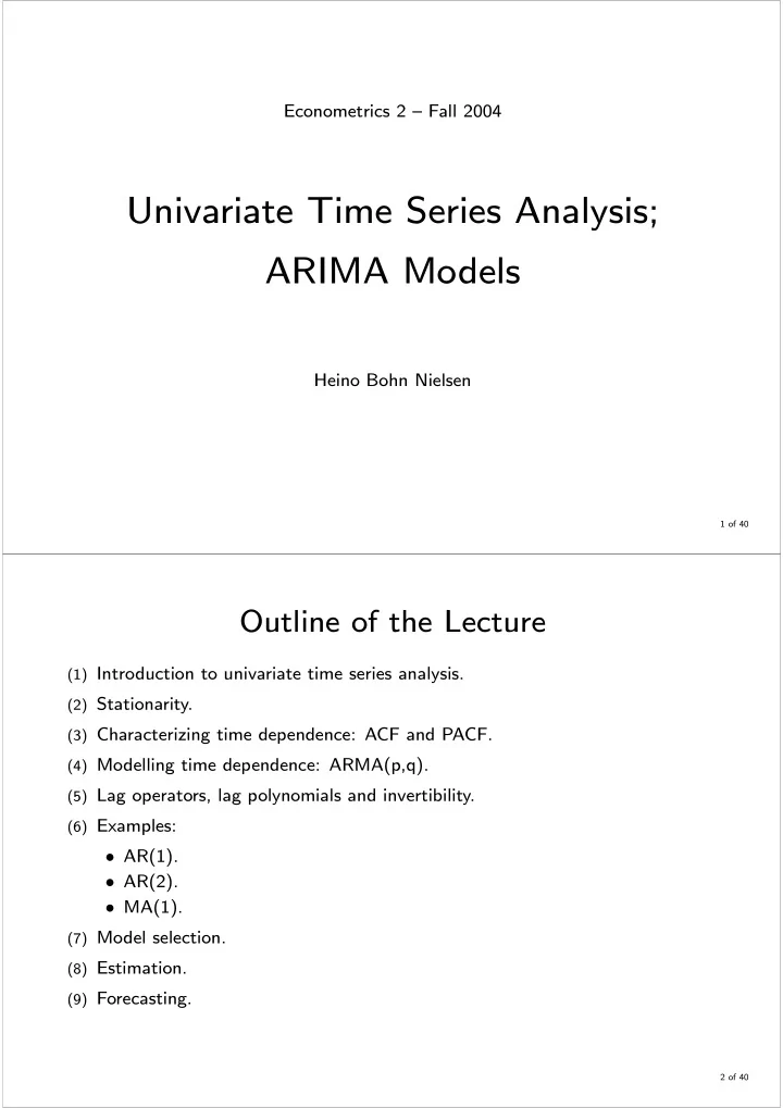
Econometrics 2 — Fall 2004 Univariate Time Series Analysis; ARIMA Models Heino Bohn Nielsen 1 of 40 Outline of the Lecture (1) Introduction to univariate time series analysis. (2) Stationarity. (3) Characterizing time dependence: ACF and PACF. (4) Modelling time dependence: ARMA(p,q). (5) Lag operators, lag polynomials and invertibility. (6) Examples: • AR(1). • AR(2). • MA(1). (7) Model selection. (8) Estimation. (9) Forecasting. 2 of 40

Univariate Time Series Analysis • Consider a single time series: y 1 , y 2 , ..., y T . Simple models for y t as a function of the past. • Univariate models are used for — Analyzing the properties of a time series. The dynamic adjustment after a chock. Transitory or permanent e ff ects. Presence of unit roots. — Forecasting. A model for E [ y t | x t ] is only useful for forecasting y t +1 if we know (or can forecast) x t +1 . — Introducing the tools necessary for analyzing more complicated models. 3 of 40 Stationarity • A time series, y 1 , y 2 , ..., y t , ..., y T , is (strictly) stationary if the joint distributions ( y t 1 , y t 2 , ..., y t n ) and ( y t 1 + h , y t 2 + h , ..., y t n + h ) are the same for all h . • A time series is called weakly stationary or covariance stationary if E [ y t ] = µ V [ y t ] = E [( y t − µ ) 2 ] = γ 0 Cov [ y t , y t − k ] = E [( y t − µ ) ( y t − k − µ )] = γ k for k = 1 , 2 , ... Often µ and γ 0 are assumed fi nite. • On these slides we consider only stationary processes. Later we consider non-stationary processes. 4 of 40

The Autocorrelation Function (ACF) • For a stationary time series we de fi ne the autocorrelation function (ACF) as à ! = Cov ( y t , y t − k ) Cov ( y t , y t − k ) ρ k = Corr ( y t , y t − k ) = γ k p , = . γ 0 V ( y t ) V ( y t ) · V ( y t − k ) Note that − 1 ≤ ρ k ≤ 1 , ρ 0 = 1 , and ρ k = ρ − k . • Recall that the ACF can (e.g.) be estimated by OLS in the regression model y t = c + ρ k y t − k + residual. • Under the assumption of white noise, ρ 1 = ρ 2 = ... = 0 , it holds that ρ k ) = T − 1 , V ( b √ and 95% con fi dence bands are given by ± 2 / T . 5 of 40 The Partial Autocorrelation Function (PACF) • An alternative measure is the partial autocorrelation function (PACF), which is the correlation conditional on the intermediate values, i.e. Corr ( y t , y t − k | y t − 1 , ..., y t − k +1 ) . • The PACF can be estimated as the OLS estimator b θ k in the regression y t = c + θ 1 y t − 1 + ... + θ k y t − k + residual, where the intermediate lags are included. • Under the assumption of white noise, θ 1 = θ 2 = ... = 0 , it holds that V ( b θ k ) = T − 1 . √ 95% con fi dence bands are given by ± 2 / T . 6 of 40

(A) Danish income, log of constant prices (B) Deviation from trend 6.4 2 6.2 0 6.0 1970 1980 1990 2000 1970 1980 1990 2000 (C) Estimated ACF (D) Estimated PACF 1 1 0 0 0 5 10 15 20 0 5 10 15 20 7 of 40 The ARMA(p,q) Model • We consider two simple models for y t : The autoregressive AR(p) model and the moving average MA(q) model. • First de fi ne a white noise process, � t ∼ i.i.d. (0 , σ 2 ) . • The AR(p) model is de fi ned as y t = θ 1 y t − 1 + θ 2 y t − 2 + ... + θ p y t − p + � t . Systematic part of y t is a linear function of p lagged values. • The MA(q) model is de fi ned as y t = � t + α 1 � t − 1 + α 2 � t − 2 + ... + α q � t − q . y t is a moving average of past chocks to the process. • They can be combined into the ARMA(p,q) model y t = θ 1 y t − 1 + ... + θ p y t − p + � t + α 1 � t − 1 + ... + α q � t − q . 8 of 40

The Lag— and Di ff erence Operators • De fi ne the lag-operator, L , to have the property that Ly t = y t − 1 . Note, that L 2 y t = L ( Ly t ) = Ly t − 1 = y t − 2 . • Also de fi ne the fi rst di ff erence operator, ∆ = 1 − L , such that ∆ y t = (1 − L ) y t = y t − Ly t = y t − y t − 1 . Note, that ∆ 2 y t = ∆ ( ∆ y t ) = ∆ ( y t − y t − 1 ) = ∆ y t − ∆ y t − 1 = ( y t − y t − 1 ) − ( y t − 1 − y t − 2 ) = y t − 2 y t − 1 + y t − 2 . 9 of 40 Lag Polynomials • Consider as an example the AR(2) model y t = θ 1 y t − 1 + θ 2 y t − 2 + � t . That can be written as y t − θ 1 y t − 1 − θ 2 y t − 2 = � t (1 − θ 1 L − θ 2 L 2 ) y t = � t θ ( L ) y t = � t , where θ ( L ) = 1 − θ 1 L − θ 2 L 2 is a polynomial in L denoted a lag-polynomial. • Standard rules for calculating with polynomials also hold for polynomials in L . 10 of 40

Characteristic Equations and Roots • For a model y t − θ 1 y t − 1 − θ 2 y t − 2 = θ ( L ) y t = � t , we de fi ne the characteristic equation as θ ( z ) = 1 − θ 1 z − θ 2 z 2 = 0 . The solutions, z 1 and z 2 , are denoted characteristic roots. • An AR(p) has p roots. Some of them may be complex values, h ± v · i , where i = √− 1 . • The roots can be used for factorizing the polynomial θ ( z ) = 1 − θ 1 z − θ 2 z 2 = (1 − φ 1 z ) (1 − φ 2 z ) , where φ 1 = z − 1 and φ 2 = z − 1 2 . 1 11 of 40 Invertibility of Polynomials • De fi ne the inverse of a polynomial, θ − 1 ( L ) of θ ( L ) , so that θ − 1 ( L ) θ ( L ) = 1 . • Consider the AR(1) case, θ ( L ) = 1 − θL , and look at the product ¡ 1 + θL + θ 2 L 2 + θ 3 L 3 + ... + θ k L k ¢ (1 − θL ) ¡ θL − θ 2 L 2 ¢ ¡ θ 2 L 2 − θ 3 L 3 ¢ ¡ θ 3 L 3 − θ 4 L 5 ¢ = (1 − θL ) + + + + ... = 1 − θ k +1 L k +1 . If | θ | < 1 , it holds that θ k +1 L k +1 → 0 as k → ∞ implying that X ∞ 1 θ − 1 ( L ) = (1 − θL ) − 1 = 1 − θL = 1 + θL + θ 2 L 2 + θ 3 L 3 + ... = θ i L i i =0 • If θ ( L ) is a fi nite polynomial, the inverse polynomial, θ − 1 ( L ) , is in fi nite. 12 of 40

ARMA Models in AR and MA form • Using lag polynomials we can rewrite the stationary ARMA(p,q) model as y t − θ 1 y t − 1 − ... − θ p y t − p = � t + α 1 � t − 1 + ... + α q � t − q ( ∗ ) θ ( L ) y t = α ( L ) � t . where θ ( L ) and α ( L ) are fi nite polynomials. • If θ ( L ) is invertible, ( ∗ ) can be written as the in fi nite MA( ∞ ) model y t = θ − 1 ( L ) α ( L ) � t y t = � t + γ 1 � t − 1 + γ 2 � t − 2 + ... This is called the MA representation. • If α ( L ) is invertible, ( ∗ ) can be written as an in fi nite AR( ∞ ) model α − 1 ( L ) θ ( L ) y t = � t y t − γ 1 y t − 1 − γ 2 y t − 2 − ... = � t . This is called the AR representation. 13 of 40 Invertibility and Stationarity • A fi nite order MA process is stationary by construction. — It is a linear combination of stationary white noise terms. — Invertibility is sometimes convenient for estimation and prediction. • An in fi nite MA process is stationary if the coe ffi cients, α i , converge to zero. — We require that P ∞ i =1 α 2 i < ∞ . • An AR process is stationary if θ ( L ) is invertible. — This is important for interpretation and inference. — In the case of a root at unity standard results no longer hold. We return to unit roots later. 14 of 40

• Consider again the AR(2) model θ ( z ) = 1 − θ 1 z − θ 2 z 2 = (1 − φ 1 L ) (1 − φ 2 L ) . The polynomial is invertible if the factors (1 − φ i L ) are invertible, i.e. if | φ 1 | < 1 | φ 2 | < 1 . and • In general a polynomial, θ ( L ) , is invertible if the characteristic roots, z 1 , ..., z p , are larger than one in absolute value. In complex cases, this corresponds to the roots being outside the complex unit circle. (Modulus larger than one). 15 of 40 ARMA Models and Common Roots • Consider the stationary ARMA(p,q) model y t − θ 1 y t − 1 − ... − θ p y t − p = � t + α 1 � t − 1 + ... + α q � t − q θ ( L ) y t = α ( L ) � t ¡ ¢ ¡ ¢ (1 − φ 1 L ) (1 − φ 2 L ) · · · 1 − φ p L y t = (1 − ξ 1 L ) (1 − ξ 2 L ) · · · 1 − ξ q L � t . • If φ i = ξ j for some i, j , they are denoted common roots or canceling roots. The ARMA(p,q) model is equivalent to a ARMA(p-1,q-1) model. • As an example, consider y t − y t − 1 + 0 . 25 y t − 2 = � t − 0 . 5 � t − 1 ¡ 1 − L + 0 . 25 L 2 ¢ y t = (1 − 0 . 5 L ) � t (1 − 0 . 5 L ) (1 − 0 . 5 L ) y t = (1 − 0 . 5 L ) � t (1 − 0 . 5 L ) y t = � t . 16 of 40

Unit Roots and ARIMA Models • A root at one is denoted a unit root, and has important consequences for the analysis. We consider tests for unit roots and unit root econometrics later. • Consider an ARMA(p,q) model θ ( L ) y t = α ( L ) � t . If there is a unit root in the AR polynomial, we can factorize into ¡ ¢ = (1 − L ) θ ∗ ( L ) , θ ( L ) = (1 − L ) (1 − φ 2 L ) · · · 1 − φ p L and we can write the model as θ ∗ ( L )(1 − L ) y t = α ( L ) � t θ ∗ ( L ) ∆ y t = α ( L ) � t . • An ARMA(p,q) model for ∆ d y t is denoted an ARIMA(p,d,q) model for y t . 17 of 40 Example: Danish Real House Prices • Consider the Danish real house prices in logs, p t . An AR(2) model yields p t = 1 . 551 p t − 1 − 0 . 5734 p t − 2 + 0 . 003426 (20 . 7) ( − 7 . 56) (1 . 30) The lag polynomial is given by θ ( L ) = 1 − 1 . 551 · L + 0 . 5734 · L 2 , with inverse roots given by 0 . 9422 and 0 . 6086 . • One root is close to unity and we estimate an ARIMA(2,1,0) model for p t : ∆ p t = 1 . 323 ∆ p t − 1 − 0 . 4853 ∆ p t − 2 + 0 . 0009959 (16 . 6) ( − 6 . 12) (0 . 333) The lag polynomial is given by θ ( L ) = 1 − 1 . 323 · L + 0 . 4853 · L 2 , with complex (inverse) roots given by √ 0 . 66140 ± 0 . 21879 · i, where i = − 1 . 18 of 40