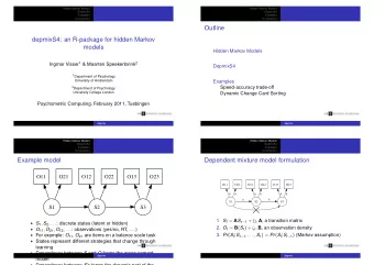
Hidden Markov Models Slides adapted from Joyce Ho, David Sontag, - PowerPoint PPT Presentation

Hidden Markov Models Slides adapted from Joyce Ho, David Sontag, Geoffrey Hinton, Eric Xing, and Nicholas Ruozzi

Sequential Data • Time-series: Stock market, weather, speech, video • Ordered: Text, genes

Sequential Data: Tracking Observe noisy measurements of missile location Where is the missile now? Where will it be in 1 minute?

Sequential Data: Weather • Predict the weather tomorrow using previous information • If it rained yesterday, and the previous day and historically it has rained 7 times in the past 10 years on this date — does this affect my prediction?

Sequential Data: Weather • Use product rule for joint distribution of a sequence • How do I solve this? • Model how weather changes over time • Model how observations are produced • Reason about the model

Markov Chain • Set S is called the state space • Process moves from one state to another generating a sequence of states: x 1 , x 2 , …, x t • Markov chain property: probability of each subsequent state depends only on the previous state:

Markov Chain: Parameters State transition matrix A (|S| x |S|) • A is a stochastic matrix (all rows sum to one) Time homogenous Markov chain: transition probability between two states does not depend on time Initial (prior) state probabilities •

Example of Markov Model 0.3 0.7 Rain Dry 0.2 0.8 • Two states : ‘Rain’ and ‘Dry’. • Transition probabilities: P (‘Rain’|‘Rain’)= 0.3, P(‘Dry’|‘Rain’)= 0.7 P (‘Rain’|‘Dry’) =0.2, P(‘Dry’|‘Dry’)=0.8 • Initial probabilities: P (‘Rain’)=0.4 , P(‘Dry’)= 0.6

Example: Weather Prediction Compute probability of tomorrow’s • weather using Markov property Evaluation: given today is dry, what’s • the probability that tomorrow is dry and the next day is rainy? P({‘Dry’,’Dry’,’Rain’} ) = P (‘Rain’|’Dry’) P(‘Dry’|’Dry’) P(‘Dry’) = 0.2*0.8*0.6 Learning: give some observations, • determine the transition probabilities

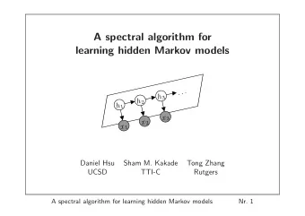
Hidden Markov Model (HMM) • Stochastic model where the states of the model are hidden • Each state can emit an output which is observed

HMM: Parameters • State transition matrix A • Emission / observation conditional output probabilities B • Initial (prior) state probabilities

Example of Hidden Markov Model 0.3 0.7 Low High 0.2 0.8 0.6 0.6 0.4 0.4 Rain Dry

Example of Hidden Markov Model • Two states : ‘Low’ and ‘High’ atmospheric pressure. • Two observations : ‘Rain’ and ‘Dry’. • Transition probabilities: P (‘Low’|‘Low’)=0.3 , P(‘High’|‘Low’)= 0.7 P (‘Low’|‘High’)=0.2, P(‘High’|‘High’)=0.8 • Observation probabilities : P (‘Rain’|‘Low’)=0.6 , P(‘Dry’|‘Low’)=0.4 P (‘Rain’|‘High’)=0.4 , P(‘Dry’|‘High’)= 0.3 • Initial probabilities: P (‘Low’)=0.4 , P(‘High’)= 0.6

Calculation of observation sequence probability • Suppose we want to calculate a probability of a sequence of observations in our example, {‘Dry’,’Rain’}. • Consider all possible hidden state sequences: P({‘Dry’,’Rain’} ) = P({‘Dry’,’Rain’} , {‘Low’,’Low’}) + P({‘Dry’,’Rain’} , {‘Low’,’High’}) + P({‘Dry’,’Rain’} , {‘High’,’Low’}) + P({‘Dry’,’Rain’} , {‘High’,’High’}) where first term is : P({‘Dry’,’Rain’} , {‘Low’,’Low’})= P({‘Dry’,’Rain’} | {‘Low’,’Low’}) P({‘Low’,’Low’}) = P(‘Dry’|’Low’)P(‘Rain’|’Low’) P(‘Low’)P(‘Low’|’Low ) = 0.4*0.4*0.6*0.4*0.3

Example: Dishonest Casino • A casino has two dices that it switches between with 5% probability • Fair dice • Loaded dice

Example: Dishonest Casino • Initial probabilities • State transition matrix • Emission probabilities

Example: Dishonest Casino • Given a sequence of rolls by the casino player • How likely is this sequence given our model of how the casino works? – evaluation problem • What sequence portion was generated with the fair die, and what portion with the loaded die? – decoding problem • How “loaded” is the loaded die? How “fair” is the fair die? How often does the casino player change from fair to loaded and back? – learning problem

HMM: Problems Evaluation : Given parameters and observation sequence, • find probability ( likelihood ) of observed sequence - forward algorithm Decoding : Given HMM parameters and observation • sequence, find the most probable sequence of hidden states - Viterbi algorithm Learning : Given HMM with unknown parameters and • observation sequence, find the parameters that maximizes likelihood of data - Forward-Backward algorithm

HMM: Evaluation Problem • Given • Probability of observed sequence Summing over all possible hidden state values at all times — K T exponential # terms

Trellis representation of an HMM o 1 o t o t+1 o T = Observations s 1 s 1 s 1 s 1 a 1j s 2 s 2 s 2 s 2 a 2j s i s i s j s i a ij a Kj s K s K s K s K Time= 1 t t+1 T

HMM: Forward Algorithm Instead pose as recursive problem • Dynamic program to compute forward probability in state S t = k • after observing the first t observations k k t t t Algorithm: • - initialize: t=1 - iterate with recursion: t=2, … t=k … - terminate: t=T

HMM: Problems Evaluation : Given parameters and observation sequence, • find probability ( likelihood ) of observed sequence - forward algorithm Decoding : Given HMM parameters and observation • sequence, find the most probable sequence of hidden states - Viterbi algorithm Learning : Given HMM with unknown parameters and • observation sequence, find the parameters that maximizes likelihood of data - Forward-Backward algorithm

HMM: Decoding Problem 1 • Given • Probability that hidden state at time t was k We know how to compute the first part using forward algorithm

HMM: Backward Probability • Similar to forward probability, we can express as a recursion problem k t t t • Dynamic program • Initialize • Iterate using recursion

HMM: Decoding Problem 1 • Probability that hidden state at time t was k Forward- backward algorithm • Most likely state assignment

HMM: Decoding Problem 2 • Given • What is most likely state sequence? probability of most likely sequence of states ending at state S T =k

HMM: Viterbi Algorithm • Compute probability recursively over t • Use dynamic programming again!

HMM: Viterbi Algorithm • Initialize • Iterate • Terminate Traceback

HMM: Computational Complexity • What is the running time for the forward algorithm, backward algorithm, and Viterbi? O(K 2 T) vs O(K T )!

HMM: Problems Evaluation : Given parameters and observation sequence, • find probability ( likelihood ) of observed sequence - forward algorithm Decoding : Given HMM parameters and observation • sequence, find the most probable sequence of hidden states - Viterbi algorithm Learning : Given HMM with unknown parameters and • observation sequence, find the parameters that maximizes likelihood of data - Forward-Backward, Baum-Welch algorithm

HMM: Learning Problem • Given only observations • Find parameters that maximize likelihood • Need to learn hidden state sequences as well

HMM: Baum-Welch (EM) Algorithm • Randomly initialize parameters • E-step: Fix parameters, find expected state assignment Forward-backward algorithm

HMM: Baum-Welch (EM) Algorithm • Expected number of times we will be in state i • Expected number of transitions from state i • Expected number of transitions from state i to j

HMM: Baum-Welch (EM) Algorithm • M-step: Fix expected state assignments, update parameters

HMM: Problems Evaluation : Given parameters and observation sequence, • find probability ( likelihood ) of observed sequence - forward algorithm Decoding : Given HMM parameters and observation • sequence, find the most probable sequence of hidden states - Viterbi algorithm Learning : Given HMM with unknown parameters and • observation sequence, find the parameters that maximizes likelihood of data - Forward-Backward (Baum-Welch) algorithm

HMM vs Linear Dynamical Systems • HMM • States are discrete • Observations are discrete or continuous • Linear dynamical systems • Observations and states are multivariate Gaussians • Can use Kalman Filters to solve

Linear State Space Models • States & observations are Gaussian • Kalman filter: (recursive) prediction and update

More examples • Location prediction • Privacy preserving data monitoring

Next Location Prediction: Definitions

Next Location Prediction: Classification of Methods o Personalization • Individual-based methods only utilize the history of one object to predict its future locations. • General-based methods use the movement history of other objects additionally (e.g. similar objects or similar trajectories) to predict the object’s future location. Source: A. Monreale, F. Pinelli, R. Trasarti, F. Giannotti. WhereNext: a Location Predictor on Trajectory Pattern Mining . KDD 2009