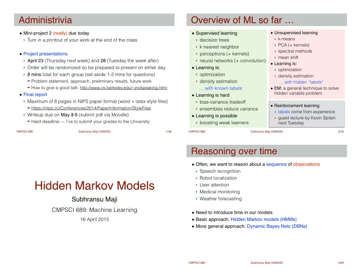
Hidden Markov Models User attention Medical monitoring Subhransu - PowerPoint PPT Presentation

Administrivia Overview of ML so far … Unsupervised learning ! Mini-project 2 (really) due today ! Supervised learning ! ‣ k-means ‣ Turn in a printout of your work at the end of the class ‣ decision trees ‣ PCA (+ kernels) ‣ k nearest neighbor ! ‣ spectral methods ‣ perceptrons (+ kernels) Project presentations ! ‣ mean shift ‣ April 23 (Thursday next week) and 28 (Tuesday the week after) ‣ neural networks (+ convolution) Learning is: ! ‣ Order will be randomized so be prepared to present on either day Learning is: ! ‣ optimization ‣ 8 mins total for each group (set aside 1-2 mins for questions) ‣ optimization ‣ density estimation ➡ Problem statement, approach, preliminary results, future work ‣ density estimation … with hidden “labels” ➡ How to give a good talk: http://www.cs.berkeley.edu/~jrs/speaking.html … with known labels EM: a general technique to solve hidden variable problem Final report ! Learning is hard ! ! ‣ Maximum of 8 pages in NIPS paper format (word + latex style files) ‣ bias-variance tradeoff Reinforcement learning ! ➡ https://nips.cc/Conferences/2014/PaperInformation/StyleFiles ‣ ensembles reduce variance ‣ labels come from experience ‣ Writeup due on May 3 6 (submit pdf via Moodle) Learning is possible ! ‣ guest lecture by Kevin Spiteri ➡ Hard deadline — I’ve to submit your grades to the University ‣ boosting weak learners next Tuesday CMPSCI 689 Subhransu Maji (UMASS) 1 /36 CMPSCI 689 Subhransu Maji (UMASS) 2 /36 Reasoning over time Often, we want to reason about a sequence of observations ! ‣ Speech recognition ‣ Robot localization Hidden Markov Models ‣ User attention ‣ Medical monitoring Subhransu Maji ‣ Weather forecasting ! CMPSCI 689: Machine Learning Need to introduce time in our models ! 16 April 2015 Basic approach: Hidden Markov models (HMMs) ! More general approach: Dynamic Bayes Nets (DBNs) CMPSCI 689 Subhransu Maji (UMASS) 4 /36

Bayes network — a quick intro Markov models A way of specifying conditional independences ! A Markov model is a chain-structured BN ! ‣ Each node is identically distributed (stationarity) A Bayes Network (BN) is a directed acyclic graph (DAG) ! ‣ Value of X at a given time t is called the state Nodes are random variables ! ‣ As a BN: A node’s distribution only depends on its parents ! Joint distribution decomposes: ! ! ! ! p ( x ) = Π i p ( x i | Parents i ) example BN ! ! A node’s value is conditionally independent of everything else given ! the value of its parents: Parameters of the model ! X 3 p ( x 3 | x 2 ) ‣ Transition probabilities or dynamics that specify how the state X 2 p ( x 2 | x 1 ) evolves over time X 1 X 6 ‣ The initial probabilities of each state p ( x 1 ) p ( x 6 | x 2 , x 5 ) p ( x 4 | x 1 ) p ( x 5 | x 4 ) X 4 X 5 CMPSCI 689 Subhransu Maji (UMASS) 5 /36 CMPSCI 689 Subhransu Maji (UMASS) 6 /36 Conditional independence Markov model: example Weather: ! ‣ States: X = {rain, sun} ‣ Transitions: ! ! ! This is a CPT ! and not a BN! Basic conditional independence: ! ! ‣ Past and future independent of the present ! ‣ Each time step only depends on the previous ! ‣ This is called the (first order) Markov property ‣ Initial distribution: 1.0 sun ! ‣ Question: What is the probability distribution after one step? Note that the chain is just a (growing) BN ! P(X 2 =sun) = P(X 2 =sun|X 1 =sun)P(X 1 =sun) + P(X 2 =sun|X 1 =rain)P(X 1 =rain) ‣ We can always use generic BN reasoning on it (if we truncate the = 0.9 x 1.0 + 0.1 x 0.0 chain) = 0.9 CMPSCI 689 Subhransu Maji (UMASS) 7 /36 CMPSCI 689 Subhransu Maji (UMASS) 8 /36

Markov model: example Mini-forward algorithm Text synthesis — create plausible looking poetry, love letters, term Question: probability of being in a state x at a time t? ! papers, etc. ! Slow answer: ! ! ‣ Enumerate all sequences of length t with end in s Typically a higher order Markov model ! ‣ Add up their probabilities: Sample word w t based on the previous n words i.e: ! X P ( X t = sun) = P ( x 1 , . . . , x t − 1 , sun) ‣ w t ~ P(w t | w t-1 , w t-2 ,…, w t-n ) x 1 ,...,x t − 1 ‣ These probability tables can be computed from lots of text ! P ( X 1 = sun) P ( X 2 = sun | X 1 = sun) . . . P ( X t = sun | X t − 1 = sun) Examples of text synthesis [A.K. Dewdney, Scientific American 1989] ! ‣ “As I've commented before, really relating to someone involves P ( X 1 = sun) P ( X 2 = rain | X 1 = sun) . . . P ( X t = sun | X t − 1 = sun) standing next to impossible.” … ‣ “ One morning I shot an elephant in my arms and kissed him.” ‣ “ I spent an interesting evening recently with a grain of salt” O (2 t − 1 ) Slide from Alyosha Efros, ICCV 1999 CMPSCI 689 Subhransu Maji (UMASS) 9 /36 CMPSCI 689 Subhransu Maji (UMASS) 10 /36 Mini-forward algorithm Example Better way: cached incremental belief updates ! From initial observation of sun ! ‣ (GM folks: this is an instance of variable elimination) ! ! ! ! ! From initial observation of rain P ( x 1 ) = known X P ( x t ) = P ( x t − 1 ) P ( x t | x t − 1 ) x t − 1 forward simulation CMPSCI 689 Subhransu Maji (UMASS) 11 /36 CMPSCI 689 Subhransu Maji (UMASS) 12 /36

Stationary distribution Web link analysis If we simulate the chain long enough ! PageRank over a web graph ! ‣ What happens? Each web page is a state ! ‣ Uncertainty accumulates Initial distribution: uniform over pages ! ‣ Eventually, we have no idea what the state is! Transitions: ! ‣ With probability c, uniform jump to a random page (dotted lines) ! ! Stationary distributions: ! ‣ With probability 1-c, follow a random outlink (solid lines) ‣ For most chains, the distribution we end up in is independent of the ! initial distribution (but not always uniform!) Stationary distribution ! ‣ This distribution is called the stationary distribution of the chain ‣ Will spend more time on highly reachable pages ! ‣ Usually, can only predict a short time out ‣ E.g. many ways to get to the Acrobat Reader download page ! ‣ Somewhat robust to link spam (but not immune) ! ‣ Google 1.0 returned the set of pages containing all your keywords in decreasing rank, now all search engines use link analysis along with many other factors CMPSCI 689 Subhransu Maji (UMASS) 13 /36 CMPSCI 689 Subhransu Maji (UMASS) 14 /36 Hidden Markov Models Example Markov chains not so useful for most agents ! ‣ Eventually you don’t know anything anymore ! ‣ Need observations to update your beliefs ! Hidden Markov Models (HMMs) ! ‣ Underlying Markov chain over states S ‣ You observe outputs (effects) at each time step ‣ As a Bayes net: An HMM is defined by: ! ‣ Initial distribution: P(X 1 ) ‣ Transitions: O(X t | X t-1 ) ‣ Emissions: P(E | X) CMPSCI 689 Subhransu Maji (UMASS) 15 /36 CMPSCI 689 Subhransu Maji (UMASS) 16 /36

Conditional independence Real HMM examples HMMs have two important independence properties: ! Speech recognition HMMs: ! ‣ Markov hidden process, future depends on past via the present ‣ Observations are acoustic signals (continuous valued) ! ‣ Current observations independent of all else given the current state ‣ States are specific positions in specific words (so, tens of thousands) ! ! ! Machine translation HMMs: ! ! ‣ Observations are words (tens of thousands) ! ! ‣ States are translation options ! ! ! Robot tracking HMMs: ! Quiz: does this mean that the observations are independent? ‣ Observations are range readings (continuous) ‣ No, correlated by the hidden state ‣ States are positions on a map (continuous) CMPSCI 689 Subhransu Maji (UMASS) 17 /36 CMPSCI 689 Subhransu Maji (UMASS) 18 /36 Filtering states Example: Robot localization Sensor model: can sense if each side has a wall or not Filtering is the task of tracking the distribution B(X) (the belief state) ! (never more than 1 mistake) We start with B(X) in the initial setting, usually uniform ! Motion model: may not execute action with a small probability As time passes, or we get observations we update B(X) prob high low t=0 Example from Michael Pfeiffer CMPSCI 689 Subhransu Maji (UMASS) 19 /36 CMPSCI 689 Subhransu Maji (UMASS) 20 /36

Example: Robot localization Example: Robot localization prob prob high low high low t=1 t=2 CMPSCI 689 Subhransu Maji (UMASS) 21 /36 CMPSCI 689 Subhransu Maji (UMASS) 22 /36 Example: Robot localization Example: Robot localization prob prob high low high low t=3 t=4 CMPSCI 689 Subhransu Maji (UMASS) 23 /36 CMPSCI 689 Subhransu Maji (UMASS) 24 /36

Example: Robot localization Passage of time Assume we have a current belief state P(X | evidence to date) ! ! ! Then, after one time step passes: ! ! ! Or, compactly: ! ! ! ! prob Basic idea: beliefs get “pushed” though the transitions ! high low ‣ With the “B” notation, we have to be careful about what time step t t=5 the belief is about, and what evidence it includes CMPSCI 689 Subhransu Maji (UMASS) 25 /36 CMPSCI 689 Subhransu Maji (UMASS) 26 /36 Example HMM Most likely explanation Question: most likely sequence ending in x at time t? ! ‣ E.g., if sun on day 4, what’s the most likely sequence? ‣ Intuitively: probably sun on all four days ! Slow answer: enumerate and score ! ! most likely sequence ← arg x 1 ,...,x t − 1 P ( x 1 , . . . , x t − 1 , sun) max ! ! O (2 t − 1 ) ‣ Complexity CMPSCI 689 Subhransu Maji (UMASS) 27 /36 CMPSCI 689 Subhransu Maji (UMASS) 28 /36