Getting to Know grid Graphics Paul Murrell, The University of - PDF document
Getting to Know grid Graphics Paul Murrell, The University of Auckland, June 2015 An overview of the short course Introduction Getting to Know grid Graphic For the book "London: The Information Capital", each infographic was begun in
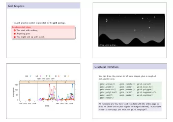
Getting to Know grid Graphics Paul Murrell, The University of Auckland, June 2015 An overview of the short course Introduction Getting to Know grid Graphic For the book "London: The Information Capital", each infographic was begun in R and then "finished off" in Adobe Illustrator. This sort of thing bugs me because I have a deep need to do all of my drawing in code (for keeping a record and for replication and for sharing, among other things).
Introduction One of the distinguishing features of the R graphics system, and the 'grid' graphics system in particular, is that it allows you fine control over details, including access to more advanced graphical features and details. As a "dramatic" demonstration of this idea, the image on this slide was generated completely in R. This course will try to reveal how 'grid' works so that you can do this sort of thing yourself. Where is grid ? The 'grid' package provides an ALTERNATIVE graphics system to the 'graphics' package ("base" graphics). Many packages define plotting functions based on 'graphics', but there are some important ones based on 'grid', such as 'lattice' and 'ggplot2'.
Where is grid ? library(lattice) xyplot(mpg ~ disp, mtcars) When you draw a plot with 'lattice' or 'ggplot2', the actual drawing is being done by 'grid'. Exploring grid Grobs library(grid) grid.ls() plot_01.background plot_01.xlab plot_01.ylab plot_01.ticks.top.panel.1.1 plot_01.ticks.left.panel.1.1 plot_01.ticklabels.left.panel.1.1 plot_01.ticks.bottom.panel.1.1 plot_01.ticklabels.bottom.panel.1.1 plot_01.ticks.right.panel.1.1 plot_01.xyplot.points.panel.1.1 plot_01.border.panel.1.1 When you draw something with 'grid', a record is kept of the objects that are drawn. 'grid' calls these objects "grobs" (graphical objects). The grid.ls() function can be used to list the grobs on the current page. Exploring grid Grobs Some other functions that help with exploring grobs: grid.grep(path) Search for a grob that matches 'path'. showGrob(gPath) Highlight grob that matches 'gPath'. SVG version with grob names as tooltips grobBrowser() (from the 'gridDebug' package).
grid Viewports xyplot(mpg ~ disp, mtcars) When you draw something with 'grid', a record is also kept of any "viewports" that were created. A viewport is a rectangular sub-region on the page. Exploring grid Viewports current.vpTree() viewport[ROOT] viewport[plot_01.toplevel.vp] viewport[plot_01.xlab.vp] viewport[plot_01.panel.1.1.vp] viewport[plot_01.panel.1.1.off.vp] viewport[plot_01.strip.left.1.1.off.vp] viewport[plot_01.ylab.vp] viewport[plot_01.figure.vp] viewport[plot_01.] viewport[plot_01.strip.1.1.off.vp] The current.vpTree() function can be used to list the viewports on the current page. Unfortunately, the output is pretty messy, but hopefully I have shared with you a little function called formatVPTree() that tidies the output up (the tidied output is shown above). Exploring grid Viewports grid.ls(viewports=TRUE, grobs=FALSE) ROOT plot_01.toplevel.vp plot_01.xlab.vp plot_01.ylab.vp plot_01.figure.vp plot_01.panel.1.1.vp plot_01.strip.1.1.off.vp plot_01.strip.left.1.1.off.vp plot_01.panel.1.1.off.vp The grid.ls() function can also be used to list the viewports on the current page. (The output on this slide has been trimmed and tidied to fit on one slide.)
Exploring grid Viewports grid.ls(viewports=TRUE, fullNames=TRUE) viewport[ROOT] rect[plot_01.background] viewport[plot_01.toplevel.vp] viewport[plot_01.xlab.vp] text[plot_01.xlab] upViewport[1] viewport[plot_01.ylab.vp] text[plot_01.ylab] upViewport[1] viewport[plot_01.figure.vp] This is the first few lines of the complete output from grid.ls() that shows both viewports and grobs (and therefore the nesting of grobs within viewports). Exploring grid Viewports Some other functions that help with exploring viewports: Highlight viewport that matches 'vp'. showViewport(vp) current.viewport() Returns the current viewport. Ideally, a package will document the naming scheme that it uses for grobs and viewports. Ideally, a package will have a naming scheme! Exercise The purpose of this exercise is to make use of the grid.ls() function. The following code creates a 'lattice' scatterplot: library(lattice) xyplot(mpg ~ disp, mtcars, main="Fast Cars") 1. What is the name of the grob that represents the main title on the scatterplot ? 2. What is the name of the viewport that the main title is drawn within ?
Why Grobs ? library(lattice) barchart(Party ~ Amount_Donated, sortedTotals) One benefit of having access to the low-level 'grid' grobs is that we can make detailed customisations to a plot that was drawn with a high-level function where the high-level function does not provide control over enough of the details. In this case, I want to remove the border around the lattice panel. Why Grobs ? library(grid) grid.ls() plot_01.background plot_01.xlab plot_01.ticks.top.panel.1.1 plot_01.ticklabels.left.panel.1.1 plot_01.ticks.bottom.panel.1.1 plot_01.ticklabels.bottom.panel.1.1 plot_01.abline.v.panel.1.1 plot_01.barchart.abline.v.panel.1.1 plot_01.barchart.rect.panel.1.1 plot_01.border.panel.1.1 If I can find out what the grob is called ...
Why Grobs ? library(grid) grid.remove("plot_01.border.panel.1.1") ... then I can remove it with grid.remove(). Working With Grobs Functions that can be used to access grobs: grid.remove() Remove a grob. Modify a grob component. grid.edit() Get a copy of a grob component. grid.get() Replace a grob component. grid.set() Each function takes the name of a grob as its first argument. The name argument can be a regular expression, if you specify 'grep=TRUE'. You can work with more than one grob at once if you specify 'global=TRUE'. Modifying Grobs library(grid) t <- grid.get("plot_01.ticklabels.bottom.panel.1.1") names(t) [1] "label" "x" "y" "just" [5] "hjust" "vjust" "rot" "check.overlap" [9] "name" "gp" "vp" t$just [1] "centre" "top" Grobs are just lists with components.
Modifying Grobs library(grid) grid.edit("plot_01.ticklabels.bottom.panel.1.1", just=c("left", "top")) We can use grid.edit() to change the value of a component. However, we may NOT edit 'name' or 'vp' components of a grob. Modifying Grobs library(grid) gpar(col="blue", lwd=3, lty="dashed") $col [1] "blue" $lwd [1] 3 $lty [1] "dashed" The value of the 'gp' component of a grob is created with the gpar() function.
Modifying Grobs Common gpar() settings: col (border) colour. fill fill colour. lty line type. lwd line width. cex text size multiplier. The other gpar() settings: The size of text (in points). fontsize lineheight Vertical height of a line of text (multiplier). For vertical positioning of multi-line text. "plain", "bold", "italic", or "bolditalic". fontface fontfamily "sans", "serif", "mono", or the name of a font family that makes sense on the current graphics device. "round", "square", or "butt". The shape used at the end of lines. lineend "round", "mitre", "bevel". The shape used at line corners. linejoin linemitre Number used to decide when mitre joins become bevel joins. Line expansion multiplier (affects line width). lex Modifying Grobs library(grid) grid.edit("plot_01.ticklabels.bottom.panel.1.1", gp=gpar(col="grey")) Modifying the 'gp' component of a grob ONLY changes the gpar() settings that are given new values.
Exercise The purpose of this exercise is to make use of the grid.edit() and grid.remove() functions. The following code creates a 'lattice' scatterplot: library(lattice) xyplot(mpg ~ disp, mtcars, main="Fast Cars") 1. Change the colour of the main title to red. 2. Remove the main title from the plot. Why Viewports ? Credit: John G. Bullock, Yale University. John Bullock made use of the 'lattice' viewports that were created in this multi-panel plot to centre the text below each row of plots. (He did not use the 'xlab' argument to xyplot() because he wanted greater control over the vertical placement of the text.)
Why Viewports ? Credit: John G. Bullock, Yale University. John could do this because it is possible to revisit the viewports that are created when a plot is drawn with 'grid'. Navigating Viewports xyplot(mpg ~ disp, mtcars) When you draw something with 'grid', a record is kept of any "viewports" that were created. A viewport is a rectangular sub-region on the page.
Navigating Viewports current.vpTree() viewport[ROOT] viewport[plot_01.toplevel.vp] viewport[plot_01.xlab.vp] viewport[plot_01.panel.1.1.vp] viewport[plot_01.panel.1.1.off.vp] viewport[plot_01.strip.left.1.1.off.vp] viewport[plot_01.ylab.vp] viewport[plot_01.figure.vp] viewport[plot_01.] viewport[plot_01.strip.1.1.off.vp] Viewports can be nested within each other. Navigating Viewports Viewports can be nested within each other.
Recommend
More recommend
Explore More Topics
Stay informed with curated content and fresh updates.
