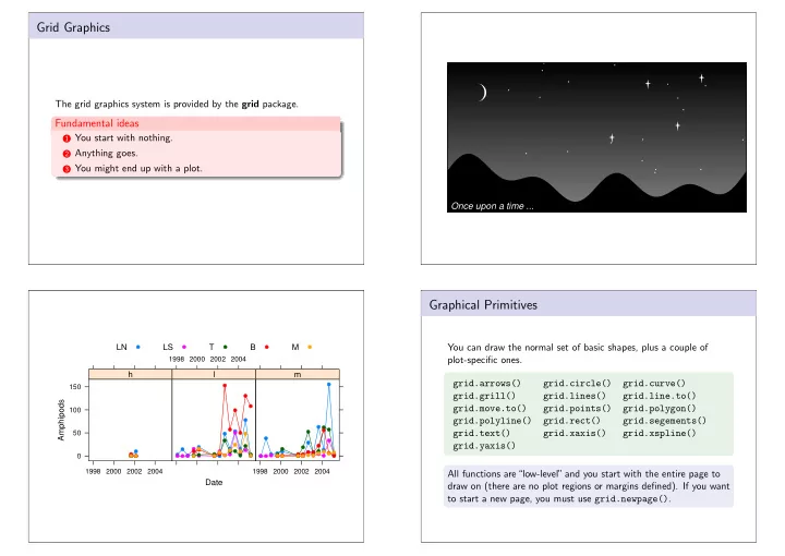
Grid Graphics The grid graphics system is provided - PowerPoint PPT Presentation

Grid Graphics ● ● ● ● ● ● ● ● ● The grid graphics system is provided by the grid package. ● Fundamental ideas 1 You start with nothing. ● ● ● 2 Anything goes. ● ● ● 3 You might end up with a plot. ● ● ● ● Once upon a time ... Graphical Primitives You can draw the normal set of basic shapes, plus a couple of LN LS T B M ● ● ● ● ● plot-specific ones. 1998 2000 2002 2004 h l m grid.arrows() grid.circle() grid.curve() ● ● 150 grid.grill() grid.lines() grid.line.to() ● Amphipods ● grid.move.to() grid.points() grid.polygon() 100 ● grid.polyline() grid.rect() grid.segements() ● ● ● ● ● ● ● ● grid.text() grid.xaxis() grid.xspline() 50 ● ● ● ● ● ● ● ● grid.yaxis() ● ● ● ● ● ● ● ● ● ● ● ● ● ● ● ● ● ● ● ● ● ● ● ● ● ● ● ● ● ● ● ● ● ● ● ● ● ● ● ● ● ● ● ● ● ● ● ● ● ● ● ● ● ● ● ● ● ● ● ● ● ● ● ● ● ● ● 0 ● ● ● ● ● ● ● ● ● ● ● ● ● ● ● ● ● ● ● ● ● ● ● ● ● ● ● ● ● ● ● ● ● ● 1998 2000 2002 2004 1998 2000 2002 2004 All functions are“low-level”and you start with the entire page to Date draw on (there are no plot regions or margins defined). If you want to start a new page, you must use grid.newpage() .

Graphical Parameters Units Drawing can be positioned and sized relative to a number of different coordinate systems . You can control the appearance of output using graphical parameters. npc , inches , cm , mm , points , char , lines . col fill alpha lty The unit() function lwd lex lineend linejoin The unit() function is used to associate a value with a coordinate linemitre fontsize cex fontfamily system. fontface lineheight font unit(1, "mm") gpar() and gp unit(1:4, "mm") The gpar() function is used to create a graphical context and unit(1:4, c("npc", "mm", "native", "lines")) the gp argument is used to apply that context to output. Working with units grid.rect(gp=gpar(col="red", fill="white", lwd=3)) It is possible to perform basic operations on units, such as addition, subtraction, calculating the maximum value, and so on. Units Viewports Unit example grid.rect(x=unit(0.4, "npc"), y=unit(1, "inches"), Drawing is always relative to the current viewport , which starts width=stringWidth("very snug"), off as the whole“page” . height=unit(1, "lines"), just=c("left", "bottom")) viewport() and pushViewport() You can define new viewports using the viewport() function. You can make your viewport the current viewport using the pushViewport() function. 0.4npc very snug It is possible to force drawing to be clipped to the viewport. 1 inch

Viewport Navigation pushViewport(viewport(width=0.8, height=0.5, angle=10, name="vp1")) grid.rect() grid.text("top-left corner", x=unit(1, "mm"), y=unit(1, "npc") - unit(1, "mm"), There are two ways to“leave”a viewport: one more destructive just=c("left", "top")) than the other. If you don’t destroy a viewport, you can revisit it pushViewport(viewport(width=0.8, height=0.5, angle=10, later. name="vp2")) popViewport() , upViewport() , and downViewport() grid.rect() grid.text("top-left corner", x=unit(1, "mm"), If you“pop”a viewport, subsequent drawing occurs in the viewport y=unit(1, "npc") - unit(1, "mm"), that existed before you pushed the viewport. The same thing just=c("left", "top")) happens if you go“up”from a viewport, but in this case the viewport is left in place and you can go back“down”to it. Functions that draw complex plots may leave their viewports intact e r to assist in further annotation. r n c o f t l e p − o t e r n r o c f t e l − p o t Layouts upViewport() grid.text("bottom-right corner", y=unit(1, "mm"), x=unit(1, "npc") - unit(1, "mm"), just=c("right", "bottom")) A layout in grid is conceptually the same as a layout in traditional downViewport("vp2") graphics, but grid layouts are more flexible and are applied in a grid.rect(width=unit(1, "npc") + unit(2, "mm"), different way. height=unit(1, "npc") + unit(2, "mm")) popViewport() grid.layout and layout.pos.col/row # downViewport("vp2") gives error! A viewport can be given a layout using grid.layout ; this divides up the viewport into rows and columns. Subsequent viewports can occupy cells in that layout using layout.pos.col/row . r n e o r c A layout in grid can make use of many different units to specify f t − l e p t o r e n o r column widths and row heights. c t f e e r − l r n c o p t o g h t − r i m o o t t b

Graphical Parameters in Viewports pushViewport(viewport(layout= grid.layout(3, 2, heights=unit(c(2, 0.5, 1), c("null", "lines", "null")), respect=TRUE))) As well as providing a geometric context for drawing, a viewport pushViewport(viewport(layout.pos.col=1, provides a graphical context for drawing. layout.pos.row=1)) The gp argument in viewport() upViewport() Graphical parameter settings in a viewport apply to all subsequent pushViewport(viewport(layout.pos.row=3)) graphical primitives and viewports, unless explicitly overridden. Some graphical parameters, such as cex , lex , and alpha are “cumulative”(more accurately, multiplicative). (1, 1) (3, 1:2) Graphical Objects pushViewport(viewport(gp=gpar(fill="grey"))) Grid produces objects representing graphical output. grid.rect(x=0.33, height=0.7, width=0.2) Graphical object names grid.rect(x=0.66, height=0.7, width=0.2, All graphical primitives have a name argument that can be used to gp=gpar(fill="black")) identify the object associated with the drawn output. popViewport() Modifying output The grid.edit() function can be used to modify output by referring to output by the graphical object name. The grid.remove() function can be used to delete elements of a plot. Positioning and sizing output based on other output The grobX() , grobY() , grobWidth() , and grobHeight() functions can be used to specify the position or size of output based on existing output.

Graphical Objects Grid and Lattice D Grid in Lattice A Grid functions, including viewport functions, can be used within a lattice panel function. B C Lattice in Grid Using print(xyplot(...), newpage=FALSE) , you can draw a lattice plot within a grid viewport. Notes Notes