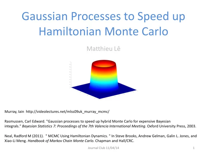
Gaussian Processes to Speed up Hamiltonian Monte Carlo Matthieu L - PowerPoint PPT Presentation
Gaussian Processes to Speed up Hamiltonian Monte Carlo Matthieu L Murray, Iain http://videolectures.net/mlss09uk_murray_mcmc/ Rasmussen, Carl Edward. "Gaussian processes to speed up hybrid Monte Carlo for expensive Bayesian
Gaussian Processes to Speed up Hamiltonian Monte Carlo Matthieu Lê Murray, Iain http://videolectures.net/mlss09uk_murray_mcmc/ Rasmussen, Carl Edward. "Gaussian processes to speed up hybrid Monte Carlo for expensive Bayesian integrals." Bayesian Statistics 7: Proceedings of the 7th Valencia International Meeting . Oxford University Press, 2003. Neal, Radford M (2011). " MCMC Using Hamiltonian Dynamics. " In Steve Brooks, Andrew Gelman, Galin L. Jones, and Xiao-Li Meng. Handbook of Markov Chain Monte Carlo . Chapman and Hall/CRC. Journal Club 11/04/14 1
MCMC • Monte Carlo : R ejection sampling, Importance sampling, … • MCMC : Markov Chain Monte Carlo • Sampling technique to estimate a probability distribution Draw samples from complex probability distributions In general : 𝑇 ∫ 𝑔 𝑦 𝑄 𝑦 𝑒𝑦 ≈ 1 𝑇 𝑔 𝑦 𝑡 𝑦 (𝑡) ~𝑄(𝑦) , 𝑡=1 Journal Club 11/04/14 2
Objective Bayesian Inference : 𝜄 : Model parameter 𝑄 𝜄 : prior on the model parameters • • 𝑄 𝑦 1 … 𝑦 𝑜 𝜄 : likelyhood, potentially expensive to evaluate • 𝑦 𝑗 : Observations • 𝑄 𝑦 1 … 𝑦 𝑜 𝜄 𝑄 𝜄 𝑄 𝜄 𝑦 1 … 𝑦 𝑜 = ∫ 𝑄 𝑦 1 … 𝑦 𝑜 𝜄 𝑄 𝜄 𝑒𝜄 𝑄 𝜄 𝑦 1 … 𝑦 𝑜 = 1 𝑎 𝑄 𝑦 1 … 𝑦 𝑜 𝜄 𝑄 𝜄 MCMC : sample 𝑄 𝜄 𝑦 1 … 𝑦 𝑜 without the knowledge of 𝑎 Journal Club 11/04/14 3
Metropolis-Hastings We want to draw samples from 𝑄 𝛽 𝑄 1. Propose new 𝜄′ from the transition function 𝑅(𝜄 ′ , 𝜄) (e.g. 𝑂 𝜄, 𝜏 2 ). The transition from one parameter to another is a Markov Chain 𝜄 ′ 𝑅(𝜄,𝜄 ′ ) 𝑄 2. Accept the new parameter 𝜄′ with a probability min (1, 𝜄 𝑅(𝜄 ′ ,𝜄) ) 𝑄 𝑅 must be chosen to fulfill some technical requirements. Samples are not independent. Sample 𝑂 0,1 ) Journal Club 11/04/14 4
Metropolis-Hastings Metropolis-Hastings: 1000 samples, step 0.1 Rejection rate: 44% Problem : The proposed samples come from a Gaussian. There is possibly an important rejection rate. Journal Club 11/04/14 5
Hamiltonian Monte Carlo Same idea as Metropolis-Hastings BUT the proposed samples now come from the Hamiltonian dynamics : 𝜖𝜄 𝜖𝑢 = 𝜖𝐹 𝑙𝑗𝑜 = 𝑞 𝑛 𝐼 = 𝐹 𝑞𝑝𝑢 + 𝐹 𝑙𝑗𝑜 𝜖𝑞 𝐹 𝑙𝑗𝑜 = 𝑞 2 𝜖𝑞 𝜖𝑢 = − 𝜖𝐹 𝑞𝑝𝑢 𝐹 𝑞𝑝𝑢 = − log 𝑄 𝜄 , 2𝑛 𝜖𝜄 𝜄 ∗ 𝜄 𝑞 𝑞 ∗ Journal Club 11/04/14 6
Hamiltonian Monte Carlo Algorithm : Sample 𝑞 according to its known distribution • • Run the Hamiltonian dynamics during a time T • Accept the new sample with probability : ∗ ∗ min (1, exp −𝐹 𝑞𝑝𝑢 + 𝐹 𝑞𝑝𝑢 exp (−𝐹 𝑙𝑗𝑜 + 𝐹 𝑙𝑗𝑜 )) The Energy is conserved so the acceptance probability should theoretically be 1. Because of the numerical precision, we need the Metropolis-Hastings type decision in the end. Journal Club 11/04/14 7
Hamiltonian Monte Carlo Gibbs Sampling Metropolis-Hastings Hamiltonian Monte Carlo Journal Club 11/04/14
Hamiltonian Monte Carlo Advantage : The Hamiltonian stays (approximately) constant during the dynamic, hence lower rejection rate ! 1000 samples, L = 200, 𝜗 =0,01 Rejection rate = 0% Problem : Computing the Hamiltonian dynamic requires computing the model partial derivatives, high number of simulation evaluation ! Neal, Radford M (2011). " MCMC Using Hamiltonian Dynamics. " In Steve Brooks, Andrew Gelman, Galin L. Jones, and Xiao-Li Meng. Handbook of Markov Chain Monte Carlo . Chapman and Hall/CRC. Journal Club 11/04/14 9
Gaussian Process HMC Same algorithm as HMC BUT the Hamiltonian dynamic is computed using Gaussian process simulating 𝐹 𝑞𝑝𝑢 𝜖𝑢 = − 𝜖𝐹 𝑞𝑝𝑢 𝜖𝑞 𝜖𝜄 Gaussian process = distribution over smooth function to approximate 𝐹 𝑞𝑝𝑢 : 𝐸 Σ pq = 𝜕 0 exp(− 1 𝑞 − 𝑦 𝑒 𝑟 2 /𝜕 𝑒 2 𝑄 𝐹 𝑞𝑝𝑢 𝜄 ~𝑂 0, Σ , 2 𝑦 𝑒 ) 𝑒=1 Journal Club 11/04/14 10
Gaussian Process HMC Once the Gaussian process is defined with a covariance matrix, we can predict new values : 𝜾, 𝑭 𝒒𝒑𝒖 , 𝜄 ∗ ~𝑂 𝜈, 𝜏 2 , ∗ 𝑄 𝐹 𝑞𝑝𝑢 If the Gaussian process is “good”, 𝜈(𝜄 ∗ ) ≈ target density Algorithm : 1. Initialization : • Evaluate the target density at D random points to define the Gaussian process. 2. Exploratory phase : HMC with 𝐹 𝑞𝑝𝑢 = 𝜈 − 𝜏 : evaluation of points with high • target value and high uncertainty. Evaluate the real target density at the end of each iteration. 3. Sampling phase : HMC with 𝐹 𝑞𝑝𝑢 = 𝜈 . • Journal Club 11/04/14 11
Gaussian Process HMC Rasmussen, Carl Edward. "Gaussian processes to speed up hybrid Monte Carlo for expensive Bayesian integrals." Bayesian Statistics 7: Proceedings of the 7th Valencia International Meeting . Oxford University Press, 2003. Journal Club 11/04/14 12
Conclusion • Metropolis-Hastings : few model evaluation per iteration but important rejection rate • Hamiltonian Monte Carlo : a lot of model evaluation per iteration but low rejection rate • GPHMC : few model evaluation per iteration and low rejection rate • BUT : Initialization requires model evaluations to define a “good” Gaussian process • BUT : Exploratory phase requires one model evaluation per iteration Journal Club 11/04/14 13
Recommend
More recommend
Explore More Topics
Stay informed with curated content and fresh updates.
