Fast Gaussian Filtering Algorithm Using Splines Kentaro Imajo (M2, - PowerPoint PPT Presentation
@imos http://imoz.jp/ /23 Fast Gaussian Filtering Algorithm Using Splines Kentaro Imajo (M2, Kyoto University) November 12, International Conference on Pattern Recognition 2012 1 /23 Contents 1. Background and Goal 2. Approximation of
@imos http://imoz.jp/ /23 Fast Gaussian Filtering Algorithm Using Splines Kentaro Imajo (M2, Kyoto University) November 12, International Conference on Pattern Recognition 2012 1
/23 Contents 1. Background and Goal 2. Approximation of Gaussian Function 3. 1D Convolution 4. 2D Convolution 5. Outline of Algorithm 6. Experiments 7. Conclusions November 12, International Conference on Pattern Recognition 2012 Chapter 0. Contents 2
/23 November 12, International Conference on Pattern Recognition 2012 Chapter 1. Background and Goal 3 Chapter 1 of 7 Background and Goal
/23 Background Many algorithms such as SIFT need to compute Gaussian filter. Chapter 1. Background and Goal November 12, International Conference on Pattern Recognition 2012 * = 2D Gaussian Func. Figure Image Blurred by 2D Gaussian Filter convolution 4
/23 Circle Gaussian Filter Chapter 1. Background and Goal November 12, International Conference on Pattern Recognition 2012 2D Gaussian Function: convolutions with 2D Gaussian function. Gaussian Filter is computed by 5 − x 2 + y 2 � � 1 2 πσ exp √ 2 σ 2 where σ is spread.
/23 Propose an algorithm to compute one Gaussian-filtered pixel Goal Chapter 1. Background and Goal November 12, International Conference on Pattern Recognition 2012 × Target Pixel 6 in constant time to area size n ( ∝ σ 2 ) . Area size is n Naïve method requires O ( n ) time.
/23 Preceding Methods but it cannot compute pixels apart. large errors. Within 3% error in constant time Chapter 1. Background and Goal November 12, International Conference on Pattern Recognition 2012 7 • Naïve method takes O ( n ) time. • FFT method is fast for all pixels, • Down-sampling method has
/23 Chapter 2. Approximation of Gaussian Function November 12, International Conference on Pattern Recognition 2012 8 Chapter 2 of 7 Approximation of Gaussian Function
/23 November 12, International Conference on Pattern Recognition 2012 Chapter 2. Approximation of Gaussian Function Spline with a spline, which is written as: Approximate Gaussian function 9 ˜ a i ( x − b i ) n � ψ ( x ) = + i where a , b , n are parameters, and ( ・ ) + is max( ・ , 0) . * Coordinates b are control points.
/23 Approximation × Gaussian func. - Approximation - × × × × 10 November 12, International Conference on Pattern Recognition 2012 Chapter 2. Approximation of Gaussian Function Control points ˜ 3( x + 11) 2 + � 11( x + 3) 2 ψ ( x ) = + +11( x � 3) 2 + � 3( x � 11) 2 + , � � 2 . 657 � 10 2 exp x 2 � � . 5 . 2720 2 240 160 80 -15 -12.5 -10 -7.5 -5 -2.5 0 2.5 5 7.5 10 12.5 15
/23 Evaluation Approximation error is about 2%. (2D error is about 3%.) Higher order improves more: Approximation error of 4 th order approximation is about 0.3%. Chapter 2. Approximation of Gaussian Function November 12, International Conference on Pattern Recognition 2012 11 ˜ 70( x + 22) 4 + − 624( x + 11) 4 + + 1331( x + 4) 4 ψ ( x ) = + − 1331( x − 4) 4 + + 624( x − 11) 4 + − 70( x − 22) 4 + .
/23 Chapter 3. 1D Convolution November 12, International Conference on Pattern Recognition 2012 12 Chapter 3 of 7 1D Convolution
/23 Chapter 3. 1D Convolution Convolution 13 November 12, International Conference on Pattern Recognition 2012 Differentiate Key Idea: Splines get discrete by differentiation. Convolution of a signal and a spline. 10 240 12 25 160 8 5 80 4 -12 -8 -4 0 4 8 12 -12 -8 -4 0 4 8 12 -12 -8 -4 0 4 8 12 -12 -8 -4 0 4 8 12 -80 -4 -5 -160 -8 -25 -240 -12 -10
/23 14 Pre-computed Transformation Several calculations Transform convolution into summation. November 12, International Conference on Pattern Recognition 2012 Chapter 3. 1D Convolution ( ˜ � ˜ ψ ∗ I )( x ) = ψ ( ∆ x ) I ( x − ∆ x ) ∆ x ∈ Z � m � � � a i ( ∆ x − b i ) n = I ( x − ∆ x ) + ∆ x ∈ Z i =0 m � � ∆ x n = a i J ( x − b i ) , J ( x ) = + I ( x − ∆ x ) i =0 ∆ x ∈ Z
/23 Chapter 4. 2D Convolution November 12, International Conference on Pattern Recognition 2012 15 Chapter 4 of 7 2D Convolution
/23 2D Convolution 20 multiplications and 16 additions 2D Gaussian func. can be decomposed: November 12, International Conference on Pattern Recognition 2012 Chapter 4. 2D Convolution 16 where Approximation can be written as: − x 2 + y 2 − x 2 − y 2 � � � � � � exp = exp exp 2 σ 2 2 σ 2 2 σ 2 m m ( ˜ � � ψ ∗ I )( x, y ) = a j J ( x − b i , y − b i ) a i i =1 j =1 J ( x, y ) = � + ∆ x n ∆ y n I ( x − ∆ x, y − ∆ y ) ( ∆ x, ∆ y ) ∈ Z 2
/23 17 Evaluation Figure Elevation and control points November 12, International Conference on Pattern Recognition 2012 Chapter 4. 2D Convolution 15 × × × × × × × × 0 y × × × × × × × × -15 -15 0 15 x · · · Gaussian — Approximation × Control point
/23 Chapter 5. Outline of Algorithm November 12, International Conference on Pattern Recognition 2012 18 Chapter 5 of 7 Outline of Algorithm
/23 Outline of Algorithm in linear time to the area of the image. 2. Compute a Gaussian filtered value in constant time (tens operations) Chapter 5. Outline of Algorithm November 12, International Conference on Pattern Recognition 2012 19 1. Pre-compute J once an image J ( x, y ) = � + ∆ x n ∆ y n I ( x − ∆ x, y − ∆ y ) ( ∆ x, ∆ y ) ∈ Z 2 for any combinations a , b. m m ( ˜ � � ψ ∗ I )( x, y ) = a j J ( x − b i , y − b i ) a i i =1 j =1
/23 Chapter 6. Experiments November 12, International Conference on Pattern Recognition 2012 20 Chapter 6 of 7 Experiments
/23 Experiments Diameter of 9 our algorithm is faster For 70+ pixels Figure Computational time for one pixel on average has 69 pixels Chapter 6. Experiments November 12, International Conference on Pattern Recognition 2012 21 10 − 4 Computational time (sec.) 10 − 5 10 − 6 10 − 7 10 − 8 10 0 10 1 10 2 10 3 10 4 # of application pixels of the filter — Proposed method - - - Na¨ ıve method
/23 Chapter 7. Conclusions November 12, International Conference on Pattern Recognition 2012 22 Final Chapter Conclusions
/23 Conclusions With pre-computing once an image, the proposed algorithm computes any size of the Gaussian filter Chapter 7. Conclusions November 12, International Conference on Pattern Recognition 2012 23 • in constant time to size, • faster than naïve for 70+ pixels, • within 3% error.
Recommend
More recommend
Explore More Topics
Stay informed with curated content and fresh updates.
