A Fast Approximation Algorithm for the Gaussian Filter Kentaro - PowerPoint PPT Presentation

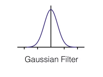
/32 A Fast Approximation Algorithm for the Gaussian Filter Kentaro Imajo (Yamamoto Laboratory) February 14, Master Thesis Defense 1

/32 I propose a fast approximation algorithm 2 Target Pixel × February 14, Master Thesis Defense Key Algorithm one Gaussian-filtered pixel for the Gaussian filter, which computes Introduction in O (1) in the area size n ( ∝ σ 2 ) . Area size is n The naïve method requires O ( n ) time.

/32 Application: Binary Classifier Extending the key algorithm, prediction of SVMs with the Gaussian kernel, with small loss of accuracy. Training (pre-computation): Prediction: February 14, Master Thesis Defense 3 Introduction • The proposed method speeds up • The proposed method speeds up training O( n 2 ) → O(4 d n log d n ) O( n ) → O(4 d log d n )

/32 Outline 1. Key Algorithm: A fast approximation algorithm for the Gaussian filter Kentaro Imajo, "Fast Gaussian Filtering Algorithm Using Splines," The 21st International Conference on Pattern Recognition, 2012. 2. Application: Binary classification Kentaro Imajo, Otaki Keisuke, Yamamoto Akihiro, "Binary Classification Using Fast Gaussian Filtering Algorithm,” Algorithms for Large-Scale Information Processing in Knowledge Discovery, 2012. 3. Conclusions February 14, Master Thesis Defense 4 Introduction

/32 February 14, Master Thesis Defense 5 Key Algorithm: Gaussian Filtering 1. Key Algorithm: Gaussian Filtering 2. Application: Binary Classification 3. Conclusions

/32 February 14, Master Thesis Defense convolution ＊ = = Summary of Key Algorithm 6 Key Algorithm: Gaussian Filtering the 2D Gaussian Function: The Gaussian filter is convolution with within 3% error. It computes one Gaussian-filtered pixel in constant time in the area size n ( ∝ σ 2 ) − x 2 + y 2 � � 1 where , the parameter σ is variance. 2 πσ exp √ 2 σ 2

/32 Problem To compute one Gaussian-filtered pixel, in the area size of the Gaussian function. compute pixels apart because FFT depends on all pixels. February 14, Master Thesis Defense 7 Key Algorithm: Gaussian Filtering • The Naïve method takes linear time • An FFT method cannot • A down-sampling method has 52% error.

/32 A spline function is a piecewise polynomial 8 February 14, Master Thesis Defense Solution function that is written as , Key Algorithm: Gaussian Filtering a discrete function is computed fast. if it is differentiated some times. using a spline function: We approximate the Gaussian function • A spline function becomes discrete – Convolution of an image and ˜ � a i ( x − b i ) n ψ ( x ) = + where ( ･ ) + is max( ･ , 0) . i

/32 Approximation Function Knots × Gaussian func. － Approximation － × × × × 9 February 14, Master Thesis Defense Key Algorithm: Gaussian Filtering ˜ 3( x + 11) 2 + � 11( x + 3) 2 ψ ( x ) = + +11( x � 3) 2 + � 3( x � 11) 2 + � � 2 . 657 � 10 2 exp x 2 � � , 5 . 2720 2 where ( ･ ) + is max( ･ , 0) . 240 160 80 -15 -12.5 -10 -7.5 -5 -2.5 0 2.5 5 7.5 10 12.5 15

/32 Approximation Function Knots × Gaussian func. － Approximation － × × × × 10 February 14, Master Thesis Defense Key Algorithm: Gaussian Filtering ˜ 3( x + 11) 2 + � 11( x + 3) 2 ψ ( x ) = + +11( x � 3) 2 + � 3( x � 11) 2 + � � 2 . 657 � 10 2 exp x 2 � � , 5 . 2720 2 where ( ･ ) + is max( ･ , 0) . 240 160 80 -15 -12.5 -10 -7.5 -5 -2.5 0 2.5 5 7.5 10 12.5 15

/32 Speed Up of Convolution This can be computed fast. Becomes DISCRETE Differentiated Integrated Key Algorithm: Gaussian Filtering 11 until it becomes discrete. The convolution can be reduced by February 14, Master Thesis Defense differentiating a spline function Intuition: ˜ ψ �� d � �� �� ( ψ ∗ I )( x ) = I ( x ) dx ( x ) dx ψ ∗

/32 The Gaussian-like approximation function Differentiate 3-times Nature of a Spline Function 12 February 14, Master Thesis Defense can also become a discrete function! Key Algorithm: Gaussian Filtering Differentiating a spline function, we can get a discrete function: 10 240 12 25 160 8 5 80 4 -12 -8 -4 0 4 8 12 -12 -8 -4 0 4 8 12 -12 -8 -4 0 4 8 12 -12 -8 -4 0 4 8 12 -80 -4 -5 -160 -8 -25 -240 -12 -10

/32 Evaluation 13 February 14, Master Thesis Defense Key Algorithm: Gaussian Filtering 4 th order approximation is about 0.3%. Higher order improves more: Approximation error is about 2%. Approximation error of | ˜ � � ( ψ ( x ) − ψ ( x ) | dx ) / ( | ψ ( x ) | dx ) ˜ 70( x + 22) 4 + − 624( x + 11) 4 + + 1331( x + 4) 4 ψ ( x ) = + − 1331( x − 4) 4 + + 624( x − 11) 4 + − 70( x − 22) 4 + .

/32 Approximation of 2D Contour lines Key Algorithm: Gaussian Filtering 14 February 14, Master Thesis Defense ˜ (3( x + 11) 2 + − 11( x + 3) 2 + + 11( x − 3) 2 + − 3( x − 11) 2 ψ ( x, y ) = + ) (3( y + 11) 2 + − 11( y + 3) 2 + + 11( y − 3) 2 + − 3( y − 11) 2 + ) 15 × × × × × × × × 0 y × × × × × × × × -15 -15 0 15 x · · · Gaussian — Approximation × Control point

/32 where The 2D Gaussian function is decomposed: 15 February 14, Master Thesis Defense 2D Convolution Key Algorithm: Gaussian Filtering The approximation can be defined as: − x 2 + y 2 − x 2 − y 2 � � � � � � exp = exp exp 2 σ 2 2 σ 2 2 σ 2 m m ( ˜ � � ψ ∗ I )( x, y ) = a j J ( x − b i , y − b j ) a i i =1 j =1 J ( x, y ) = � + ∆ x n ∆ y n I ( x − ∆ x, y − ∆ y ) ( ∆ x, ∆ y ) ∈ Z 2 O( m 2 ) linear combination , where m is # of knots for each dimension and m is equal to 4.

/32 Experiments has 69 pixels Diameter of 9 our algorithm is faster For 70+ pixels Figure Computational time for one pixel on average Key Algorithm: Gaussian Filtering February 14, Master Thesis Defense 16 10 − 4 Computational time (sec.) 10 − 5 10 − 6 10 − 7 10 − 8 10 0 10 1 10 2 10 3 10 4 # of application pixels of the filter — Proposed method - - - Na¨ ıve method

/32 Conclusions of Part 1 (1/2) We approximate the Gaussian function using a 2 nd order spline function: while general approximation functions often have equal intervals. February 14, Master Thesis Defense 17 Key Algorithm: Gaussian Filtering • It has only 2% approximation error, • It has only 4 knots, • It has unequal intervals of control points – It is sufficiently optimized as a spline.

/32 Conclusions of Part 1(2/2) … = ＊ = ＊ 18 February 14, Master Thesis Defense in constant time to the area size. we can compute every pixel apart an integrated image of an input image, Using spline approximation and Key Algorithm: Gaussian Filtering � � dx 3 dy 3

/32 February 14, Master Thesis Defense 19 Application: Binary Classification 1. Key Algorithm: Gaussian Filtering 2. Application: Binary Classification 3. Conclusions

/32 Summary of Application Extending the key algorithm, speeds up prediction of SVMs with the Gaussian kernel, with small loss of accuracy. February 14, Master Thesis Defense Judges which is nearer to 20 Application: Binary Classification • The proposed method – O( n ) → O(4 d log d n ) • It speeds up training – O( n 2 ) → O(4 d n log d n )

/32 Problem An SVM is a good binary classifier, but We cannot use SVMs if # of data gets large. Solution with small loss of accuracy. February 14, Master Thesis Defense 21 Application: Binary Classification – prediction takes O( n ) time, – training takes O( n 2 ) ～ O( n 3 ) time. • For prediction, we use the key algorithm. • For training, we treat data equally

/32 Every pixel has a value Few pixels have a value Key Algorithm It assumes that an image is given. Since we cannot integrate an image, we propose to use range trees. February 14, Master Thesis Defense 22 Image Binary Classification Application: Binary Classification

/32 Range Tree A range tree [Bentley 1979] is a data structure that February 14, Master Thesis Defense 23 Application: Binary Classification Balanced tree We can calculate the total sum with the sum can compute the total sum in a box x 1 - x 2 in O(log d n ) time with O( n log d n ) space. of O(log d n ) regions x 1 2 k x 2

/32 24 Key Algorithm The Proposed Method Range Trees Application: Binary Classification February 14, Master Thesis Defense The proposed method can decide the class of any point in O(4 d log d n ) time, and the pre-computation is O(4 d n log d n ) time. 15 × × × × × × × × 0 × × × × × × × × -15

/32 Formulation 25 February 14, Master Thesis Defense Application: Binary Classification A range tree can give: � ∆ x i ∆ y j I ( ∆ x, ∆ y ) . K i,j ( x, y ) = ( ∆ x, ∆ y ) ∈ { (0 , 0) , ··· , ( x,y ) } Using 9 range trees, J can be computed with: T   y 2    x 2  K 0 , 0 ( x, y ) K 1 , 0 ( x, y ) K 2 , 0 ( x, y )  . J ( x, y ) = − 2 y K 0 , 1 ( x, y ) K 1 , 1 ( x, y ) K 2 , 1 ( x, y ) − 2 x      1 K 0 , 2 ( x, y ) K 1 , 2 ( x, y ) K 2 , 2 ( x, y ) 1