Spatial Filtering CS/BIOEN 4640: Image Processing Basics January - PowerPoint PPT Presentation
Spatial Filtering CS/BIOEN 4640: Image Processing Basics January 31, 2012 Limitations of Point Operations They dont know where they are in an image They dont know anything about their neighbors Most image features (edges,
Spatial Filtering CS/BIOEN 4640: Image Processing Basics January 31, 2012
Limitations of Point Operations ◮ They don’t know where they are in an image ◮ They don’t know anything about their neighbors ◮ Most image features (edges, textures, etc) involve a spatial neighborhood of pixels ◮ If we want to enhance or manipulate these features, we need to go beyond point operations
What Point Operations Can’t Do Blurring/Smoothing →
What Point Operations Can’t Do Sharpening →
What Point Operations Can’t Do Weird Stuff →
Spatial Filters Definition A spatial filter is an image operation where each pixel value I ( u , v ) is changed by a function of the intensities of pixels in a neighborhood of ( u , v ) .
Example: The Mean of a Neighborhood Consider taking the mean in a 3 × 3 neighborhood: v -1 v v + 1 u -1 u u + 1 1 1 I ′ ( u , v ) = 1 � � I ( u + i , v + j ) 9 i = − 1 j = − 1
How a Linear Spatial Filter Works H is the filter “kernel” or “matrix” 1 1 1 H ( i , j ) = 1 For the neighborhood mean: 1 1 1 9 1 1 1
General Filter Equation Notice that the kernel H is just a small image! Let H : R H → [ 0 , K − 1 ] � I ′ ( u , v ) = I ( u + i , v + j ) · H ( i , j ) ( i , j ) ∈ R H This is known as a correlation of I and H
What Does This Filter Do? 0 0 0 0 1 0 0 0 0 Identity function (leaves image alone)
What Does This Filter Do? 1 1 1 1 1 1 1 9 1 1 1 Mean (averages neighborhood)
What Does This Filter Do? 0 0 0 0 0 1 0 0 0 Shift left by one pixel
What Does This Filter Do? -1 -1 -1 1 -1 17 -1 9 -1 -1 -1 Sharpen (identity minus mean filter)
Filter Normalization ◮ Notice that all of our filter examples sum up to one ◮ Multiplying all entries in H by a constant will cause the image to be multiplied by that constant ◮ To keep the overall brightness constant, we need H to sum to one � I ′ ( u , v ) = I ( u + i , v + j ) · ( cH ( i , j )) i , j � = I ( u + i , v + j ) · H ( i , j ) c i , j
Effect of Filter Size Mean Filters: 7 × 7 15 × 15 41 × 41 Original
What To Do At The Boundary?
What To Do At The Boundary? ◮ Crop
What To Do At The Boundary? ◮ Crop ◮ Pad
What To Do At The Boundary? ◮ Crop ◮ Pad ◮ Extend
What To Do At The Boundary? ◮ Crop ◮ Pad ◮ Extend ◮ Wrap
Convolution Definition Convolution of an image I by a kernel H is given by � I ′ ( u , v ) = I ( u − i , v − j ) · H ( i , j ) ( i , j ) ∈ R H This is denoted: I ′ = I ∗ H ◮ Notice this is the same as correlation with H , but with negative signs on the I indices ◮ Equivalent to vertical and horizontal flipping of H : � I ′ ( u , v ) = I ( u + i , v + j ) · H ( − i , − j ) ( − i , − j ) ∈ R H
Linear Operators Definition A linear operator F on an image is a mapping from one image to another, I ′ = F ( I ) , that satisfies: 1. F ( cI ) = cF ( I ) , 2. F ( I 1 + I 2 ) = F ( I 1 ) + F ( I 2 ) , where I , I 1 , I 2 are images, and c is a constant. Both correlation and convolution are linear operators
Infinite Image Domains Let’s define our image and kernel domains to be infinite: Ω = Z × Z Remember Z = { . . . , − 2 , − 1 , 0 , 1 , 2 , . . . } Now convolution is an infinite sum: ∞ ∞ � � I ′ ( u , v ) = I ( u − i , v − j ) · H ( i , j ) i = −∞ i = −∞ This is denoted I ′ = I ∗ H .
Infinite Image Domains The infinite image domain Ω = Z × Z is just a trick to make the theory of convolution work out. We can still imagine that the image is defined on a bounded (finite) domain, [ 0 , w ] × [ 0 , h ] , and is set to zero outside of this.
Properties of Convolution Commutativity: I ∗ H = H ∗ I This means that we can think of the image as the kernel and the kernel as the image and get the same result. In other words, we can leave the image fixed and slide the kernel or leave the kernel fixed and slide the image.
Properties of Convolution Associativity: ( I ∗ H 1 ) ∗ H 2 = I ∗ ( H 1 ∗ H 2 ) This means that we can apply H 1 to I followed by H 2 , or we can convolve the kernels H 2 ∗ H 1 and then apply the resulting kernel to I .
Properties of Convolution Linearity: ( a · I ) ∗ H = a · ( I ∗ H ) ( I 1 + I 2 ) ∗ H = ( I 1 ∗ H ) + ( I 2 ∗ H ) This means that we can multiply an image by a constant before or after convolution, and we can add two images before or after convolution and get the same results.
Properties of Convolution Shift-Invariance: Let S be the operator that shifts an image I : S ( I )( u , v ) = I ( u + a , v + b ) Then S ( I ∗ H ) = S ( I ) ∗ H This means that we can convolve I and H and then shift the result, or we can shift I and then convolve it with H .
Properties of Convolution Theorem: The only shift-invariant, linear operators on images are convolutions.
Computational Complexity of Convolution If my image I has size M × N and my kernel H has size ( 2 R + 1 ) × ( 2 R + 1 ) , then what is the complexity of convolution? R R � � I ′ ( u , v ) = I ( u − i , v − j ) · H ( i , j ) i = − R j = − R Answer: O ( MN ( 2 R + 1 )( 2 R + 1 )) = O ( MNR 2 ) . Or, if we consider the image size fixed, O ( R 2 ) .
Which is More Expensive? The following both shift the image 10 pixels to the left: 1. Convolve with a 21 × 21 shift operator (all zeros with a 1 on the right edge) 2. Repeatedly convolve with a 3 × 3 shift operator 10 times The first method requires 21 2 · wh = 441 · wh . The second method requires ( 9 · wh ) · 10 = 90 · wh .
Separability Definition A kernel H is called separable if it can be broken down into the convolution of two kernels: H = H 1 ∗ H 2 More generally, we might have: H = H 1 ∗ H 2 ∗ · · · ∗ H n Example: The “shift by ten” kernel is 10 copies of the “shift by one” kernel convolved together.
Saving Computation With Separability Remember the associative property: I ∗ ( H 1 ∗ H 2 ) = ( I ∗ H 1 ) ∗ H 2 If we can separate a kernel H into two smaller kernels H = H 1 ∗ H 2 , then it will often be cheaper to apply H 1 followed by H 2 , rather than H .
Separability in x and y Sometimes we can separate a kernel into “horizontal” and “vertical” components. Consider the kernels 1 H x = [ 1 1 1 1 1 ] , H y = 1 and 1 Then 1 1 1 1 1 H = H x ∗ H y = 1 1 1 1 1 1 1 1 1 1
Complexity of x / y -Separabile Kernels What is the number of operations for the 3 × 5 kernel H ? Answer: 15 wh What is the number of operations for H x followed by H y ? Answer: 3 wh + 5 wh = 8 wh What about the case of a M × M kernel? Answer: O ( M 2 ) – no separability ( M 2 wh operations) O ( M ) – with separability ( 2 Mwh operations)
Some More Filters Box Gaussian Laplace
A “Better” Blurring ◮ The mean (box) filter gives “blocky” blurring. ◮ We would prefer something radially symmetric. ◮ Also, blurring looks better if the weighting dies off gradually, rather than all of a sudden. ◮ The Gaussian is radially symmetric and dies off gradually.
The Gaussian In 1D: � − x 2 � 1 √ g σ ( x ) = exp 2 σ 2 2 πσ In 2D: − x 2 + y 2 � � 1 G σ ( x , y ) = 2 πσ 2 exp 2 σ 2
Separability of 2D Gaussian A 2D Gaussian is just the product of 1D Gaussians: − x 2 + y 2 � � 1 G σ ( x , y ) = 2 πσ 2 exp 2 σ 2 − x 2 − y 2 � � � � 1 1 √ √ = · exp exp 2 σ 2 2 σ 2 2 πσ 2 πσ = g σ ( x ) · g σ ( y )
Separability of 2D Gaussian As a result, convolution with a Gaussian is separable: I ∗ G = I ∗ G x ∗ G y , where G is the 2D discrete Gaussian kernel; G x is the “horizontal” and G y the “vertical” 1D discrete Gaussian kernels.
Gaussian Filtering 1. Pick a σ and radius R = 3 σ 2. Compute a 1D array (kernel) with Gaussian values k = [ g σ ( − R ) . . . g σ ( R ) ] 3. Normalize this array to sum to one 4. Convolve horizontally by k 5. Convolve vertically by k
Implementation Detail ◮ Spatial filters cannot be done “in place” ◮ Because neighbor values are needed, we can’t overwrite them ◮ Need to compute into a copy image ◮ Multiple convolutions (e.g., separable filters) need to go back and forth between two images
Recommend
More recommend
Explore More Topics
Stay informed with curated content and fresh updates.
