Shape Restricted Splines via Constrained Optimization: Computation - PowerPoint PPT Presentation

Introduction Constrained Smoothing Splines Shape Constrained Estimation via B-splines Conclusions Shape Restricted Splines via Constrained Optimization: Computation and Statistical Analysis Jinglai Shen Department of Mathematics and Statistics University of Maryland Baltimore County (UMBC), Baltimore, MD 6th Int’l Conference on Complementarity Problems Berlin, Germany, August 5, 2014 joint with Teresa Lebair (UMBC) and Xiao Wang (Purdue) Acknowledgements: J.-S. Pang (USC) and A. Draganescu (UMBC) 1 / 29

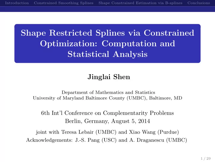
Introduction Constrained Smoothing Splines Shape Constrained Estimation via B-splines Conclusions Outline 1 Introduction 2 Constrained Smoothing Splines 3 Shape Constrained Estimation via B-splines 4 Conclusions 2 / 29

Introduction Constrained Smoothing Splines Shape Constrained Estimation via B-splines Conclusions Shape Constrained Curve-fitting/Estimation Motivation Various static or dynamic models of biologic, engineering and 1 economic systems contain shape constrained functions Example: convex shape constraint 2 1.2 True function Data 1 0.8 0.6 0.4 0 0.2 0.4 0.6 0.8 1 Applications ◮ Biology: dose response, drug combination, and genetic networks ◮ Engineering: path planning, lifetime estimation in reliability engr. ◮ Statistics: isotonic regression, log-concave density estimation 3 / 29

Introduction Constrained Smoothing Splines Shape Constrained Estimation via B-splines Conclusions Focused Topics Topic I: Computation of shape constrained smoothing splines 1 Formulated as a constrained optimal control or constrained optimization problem with nonsmooth features 2 Efficient numerical schemes Topic II: Statistical analysis of shape constrained estimators 1 Convergence of an estimator to the true function: consistency and convergence rate 2 Optimal rate estimation and minimax optimal estimation T. Robertson, F.T. Wright, and R.L. Dykstra. Order Restricted Statistical Inference . John Wiley & Sons Ltd., 1988. 4 / 29

Introduction Constrained Smoothing Splines Shape Constrained Estimation via B-splines Conclusions Smoothing Splines Smoothing spline model: unconstrained case Classical smoothing splines (Wahba): min f ∈S J ( f ), where 1 f : [0 , 1] → R , ( t i , y i ) n i =1 are samples, and � 1 � � 2 � � 2 � n J ( f ) := 1 f ( m ) ( t ) f ( t i ) − y i + λ dt n 0 i =1 Control theoretical splines (Egerstedt and Martin) 2 � 1 � � 2 � n min 1 u 2 ( t ) dt f ( t i ) − y i + λ n 0 i =1 where f ( t ) = c T x ( t ) , A ∈ R ℓ × ℓ , b, c ∈ R ℓ . x ( t ) = Ax ( t ) + bu ( t ) , ˙ � 0 � � 0 � � 1 � 1 Example: when m = 2, A = , b = , c = , and 0 0 1 0 u ( t ) = f ′′ ( t ). 5 / 29

Introduction Constrained Smoothing Splines Shape Constrained Estimation via B-splines Conclusions Shape Constrained Smoothing Splines Example: convex smoothing spline � n � � 2 + λ � 1 � � 2 dt, f (2) ≥ 0 a.e. [0 , 1] ◮ min J ( f ) := 1 f (2) ( t ) f ( t i ) − y i n i =1 0 � � 2 + λ � 1 � n ◮ equivalently, min J ( f ) := 1 0 u 2 ( t ) dt subject to f ( t i ) − y i i =1 n f ( t ) = c T x ( t ) , x ( t ) = Ax ( t ) + bu ( t ) , ˙ u ( t ) ∈ Ω := R + a.e. [0 , 1] Formulation of shape constrained smoothing spline Given a (constrained) linear control system Σ( A, B, C, Ω) on R ℓ : u ∈ W := { u ∈ L 2 ([0 , 1]; R m ) | u ( t ) ∈ Ω a.e. } , x = Ax + Bu, ˙ where A ∈ R ℓ × ℓ , B ∈ R ℓ × m , C ∈ R p × ℓ , Ω ⊆ R m is closed and convex. Given i =1 and weights w i > 0 with � n { ( t i , y i ) } n i =1 w i = 1, define the cost functional � 1 � n � � � 2 � y i − Cx ( t i ; u, x 0 ) � u ( t ) � 2 J ( u, x 0 ) := w i 2 + λ 2 dt 0 i =1 A shape constrained smoothing spline � f is determined by an optimal solution of inf J ( u, x 0 ) subject to Σ( A, B, C, Ω), i.e., � f ( t ) = Cx ( t ; u ∗ , x ∗ 0 ). 6 / 29

Introduction Constrained Smoothing Splines Shape Constrained Estimation via B-splines Conclusions Optimality Conditions Existence and uniqueness of optimal solution Suppose   Ce At 1 Ce At 2     H . 1 : rank  = ℓ.  .  .  . Ce At n 0 ) ∈ W × R ℓ for any Then there exists a unique optimal solution ( u ∗ , x ∗ ( t i , y i ), ( w i ), and λ > 0. Optimality conditions in term of VI � �� n � � � u ∗ ( t ) − λ − 1 w i P T = Π Ω i ( t ) f ( t i ) − y i , and i =1 n � � Ce A i t i � T � � � 0 = w i f ( t i ) − y i , i =1 where � f ( t i ) = Cx ( t i ; u ∗ ( t i ) , x ∗ 0 ), and P i ( t ) := Ce A ( t i − t ) B · I [0 ,t i ] . 7 / 29

Introduction Constrained Smoothing Splines Shape Constrained Estimation via B-splines Conclusions More on Optimality Conditions Facts On each [ t k , t k +1 ), u ∗ ( t ) depends on � f ( t i ) with t i < t k only. 1 0 completely determines u ∗ and � The optimal initial condition x ∗ f on 2 [0 , 1] (may write � f as � f ( t, x ∗ 0 )) Given ( t i , y i ) and ( w i ) and λ , define H y,n : R ℓ → R ℓ 3 Ce A i t i � T � � n � � � H y,n ( z ) := w i f ( t i , z ) − y i i =1 Then the equation H y,n ( z ) = 0 has a unique solution (under H . 1 ), which is the optimal initial condition x ∗ 0 . Nonsmoothness of � f ( t, · ) and H y,n If Π Ω is directionally differentiable on R m , then � f ( t, z ) is 1 B-differentiable in z for any fixed t ∈ [0 , 1]; If Π Ω is semismooth on R m , then � f ( t, z ) is semismooth in z for any 2 fixed t ∈ [0 , 1]. 8 / 29

Introduction Constrained Smoothing Splines Shape Constrained Estimation via B-splines Conclusions Boundedness of Level Sets Level set of H y,n � � z ∈ R ℓ | � H y,n ( z ) � ≤ � H y,n ( z ∗ ) � Given z ∗ ∈ R ℓ , define S z ∗ := Proposition (Boundedness of level sets) Let Ω ⊆ R m be closed and convex. For any given ( t i , y i ) , ( w i ) , λ > 0 and z ∗ such that H . 1 holds, the level set S z ∗ is bounded. Sketch of the proof Suppose not. Then there exists ( z k ) in S z ∗ with � z k � → ∞ and z k / � z k � → v ∗ � = 0. It can be shown � H y,n ( z k ) = � � lim H � y,n ( v ∗ ) y =0 , � z k � � k →∞ i =1 w i ( Ce A i t i ) T � � � y,n ( z ) = � n where � , � H � f ( t i , z ) − � y i f is obtained from the linear control system Σ( A, B, C, Ω ∞ ), and � y i = 0 , ∀ i . Since � H 0 ,n ( z ) = 0 has a unique solution z = 0, � H 0 ,n ( v ∗ ) � = 0 and � H y,n ( z k ) � → ∞ , contradiction. 9 / 29

Introduction Constrained Smoothing Splines Shape Constrained Estimation via B-splines Conclusions Solving H y,n ( z ) = 0 for Polyhedral Ω (I) Notation ◮ Define F ( z ) := B ◦ Π Ω ◦ B T ◮ For each k = 1 , 2 , . . . , n − 1, let Ce A i t � T � � � k � v k ( z ) := 1 q ( t, v ) := e − A T t v � w i f ( t i , z ) − y i , λ i =1 Then Bu ∗ ( t, z ) = F ( q ( t, v k ( z )) for all t ∈ [ t k , t k +1 ). Non-degenerate case F : R ℓ → R ℓ is continuous and piecewise affine, and admits a 1 polyhedral subdivision Ξ. For any v and k , q ( t, v ) has finitely many switchings on Ξ in [ t k , t k +1 ]. 2 q ( t, v ) is called non-degenerate on [ t k , t k +1 ] if it is in the interior of a 3 polyhedron of Ξ between any consecutive switching times; otherwise, q ( t, v ) is called degenerate. 10 / 29

Introduction Constrained Smoothing Splines Shape Constrained Estimation via B-splines Conclusions Solving H y,n ( z ) = 0 for Polyhedral Ω (II) More assumptions and notation ◮ Let ρ 1 > 0 and ρ 2 > 0 be such that � Ce A ( t − s ) � ∞ ≤ ρ 1 , ∀ t, s ∈ [0 , 1] and max i � E i � ∞ ≤ ρ 2 , where each matrix E i corresponds to an affine piece of F . ◮ Assumption H . 2 : there exist ρ t > 0 and µ ≥ ν > 0 such that for all n , 0 ≤ i ≤ n − 1 | t i +1 − t i | ≤ ρ t n ≤ w i ≤ µ ν max n , n, ∀ i. Theorem (Non-degenerate case) Let Ω be a polyhedron in R m . Assume that H . 1 − H . 2 hold and λ ≥ µ 2 ρ 2 1 ρ 2 ρ t / (4 ν ). Suppose that q ( t, v k ( z )) is non-degenerate on [ t k , t k +1 ] for each k = 1 , 2 . . . , n − 1. Then there exists a unique direction vector d ∈ R ℓ such that H y,n ( z ) + H ′ y,n ( z ; d ) = 0 . 11 / 29

Introduction Constrained Smoothing Splines Shape Constrained Estimation via B-splines Conclusions Solving H y,n ( z ) = 0 for Polyhedral Ω (III) Proposition (Degenerate case) Assume additionally that ( C, A ) is an observable pair. If q ( t, v k ( z )) is degenerate on [ t k , t k +1 ] for some k ∈ { 1 , . . . , n − 1 } , then for any ε > 0, there exists d ∈ R ℓ with 0 < � d � ≤ ε such that q ( t, v k ( z + d )) is non-degenerate on [ t k , t k +1 ] for each k = 1 , . . . , n − 1. Modified Nonsmooth Newton’s Method w. Line Search ◮ Apply the modified nonsmooth Newton’s method with line search based on (Pang, 1990) to solve H y,n ( z ) = 0 ◮ Numerical convergence is proved under suitable conditions J.-S. Pang. Newton’s method for B-differentiable equations. Mathematics of Operations Research , Vol. 15, pp. 311–341, 1990. 12 / 29