Splines linear non-linearity September 9, 2019 Splines linear - PowerPoint PPT Presentation
Splines linear non-linearity September 9, 2019 Splines linear non-linearity September 9, 2019 1 / 26 Motto A picture is worth a thousand words Splines linear non-linearity September 9, 2019 2 / 26 Fitting a non-linear
Splines – linear non-linearity September 9, 2019 Splines – linear non-linearity September 9, 2019 1 / 26
Motto “A picture is worth a thousand words” Splines – linear non-linearity September 9, 2019 2 / 26
Fitting a non-linear curve A picture 1.5 ● ● ● ● ● ● ● 1.0 ● ● ● ● ● ● ● ● ● ● 0.5 ● ● ● ● ● ● ● ● ● ● 0.0 ● Y ● ● ● ● ● ● ● ● −0.5 ● ● ● ● ● ● ● ● ● ● −1.0 ● ● −1.5 ● ● 1 2 3 4 5 6 7 8 X Try to sketch a denoised relation between X and Y . Splines – linear non-linearity September 9, 2019 4 / 26
Fitting a non-linear curve Noisy sine function Let us consider the following non-linear regression model non-linear regression Y = f ( X ) + ǫ where X is an explanatory variable, ǫ is a noisy error and Y is an outcome variable (aka response or dependent variable). The model is non-linear when f ( X ) is not a linear function of X . Consider for example f ( X ) = sin( X ) . A sample from such a model 1.5 ● ● ● ● ● ● 1.0 ● ● ● ● ● ● ● ● ● ● 0.5 ● ● ● ● ● ● ● ● ● ● ● 0.0 ● Y ● ● ● ● ● ● ● ● −0.5 ● ● ● ● ● ● ● ● ● ● −1.0 ● ● −1.5 ● ● 1 2 3 4 5 6 7 8 X Splines – linear non-linearity September 9, 2019 5 / 26
Fitting a non-linear curve Noisy Sine R-code #Non-linear regression X=runif(50,0.5,8) e=rnorm(50,0,0.35) Y=sin(X)+e pdf("NoisySine.pdf") #Save a graph to a file plot(X,Y) dev.off() #Closes the graph file Splines – linear non-linearity September 9, 2019 6 / 26
Fitting a non-linear curve How to (re-)discover a non-linear relation 1.5 ● ● ● ● ● ● ● 1.0 ● ● ● ● ● ● ● ● ● 0.5 ● ● ● ● ● ● ● ● ● ● ● 0.0 ● Y ● ● ● ● ● ● ● ● −0.5 ● ● ● ● ● ● ● ● ● ● −1.0 ● ● −1.5 ● ● 1 2 3 4 5 6 7 8 X We are now interested to recover from the above data the relation that stands behind them? In practice we do not know that there is any specific function (in this case sine function ) involved. We clearly see that the relation is non-linear. We want a standardized and automatic approach. Any ideas? Splines – linear non-linearity September 9, 2019 7 / 26
Fitting a non-linear curve Piecewise constant We first divide the domain into disjoint regions marked by the knot points ξ 0 < ξ 1 < · · · < ξ n < ξ n + 1 . ξ 0 the begining of the x -interval and ξ n + 1 its end On each interval we can fit independently. For example by constant functions Splines – linear non-linearity September 9, 2019 8 / 26
Fitting a non-linear curve Piecewise linear Where the difference between the two pictures lies? The second is continuous – a linear spline . Fit is no longer independent between regions. How to do it? Splines – linear non-linearity September 9, 2019 9 / 26
Fitting a non-linear curve Analysis of the problem How many parameters there are in the problem? 3-intercepts + 3-slopes − 2-knots = 4 (we subtract knots because each knot sets one equation to fulfill the continuity assumption) The problem should be fitted with four parameters. From now on we assume the knots locations are decided for and not changing. Splines – linear non-linearity September 9, 2019 10 / 26
Fitting a non-linear curve Making non-linear linear What is the minimal number of vectors needed to express linearly any vector in 4 dimensions? 4 Such vectors are (linearly) independent (none is linearly expressed by the remaining ones) Find 4 piecewise linear continuous functions that are ‘independent’, say h 1 ( X ) , h 2 ( X ) , h 3 ( X ) , h 4 ( X ) . Then any function piecewise linear with the given knots can be written linearly by them 4 � f ( X ) = β 1 h 1 ( X ) + β 2 h 2 ( X ) + β 3 h 3 ( X ) + β 4 h 4 ( X ) = β j h j ( X ) . j = 1 f ( X ) is continuous in X because each of h j ( X ) is. There are four parameters, so that any continuous piecewise linear function should be fitted by proper choice of β j ’s. Splines – linear non-linearity September 9, 2019 11 / 26
Fitting a non-linear curve Basis functions There many choices for h j , j = 1 , . . . , 4. The following is a natural one h 1 ( X ) = 1 , h 2 ( X ) = X , h 3 ( X ) = ( X − ξ 1 ) + , h 4 ( X ) = ( X − ξ 2 ) + , where t + is a positive part of a real number t . The model for the data Y i = β 1 h i 1 + · · · + β r h ir + ε i , i = 1 , 2 , . . . , n , where h ij = h j ( X i ) . The model in the matrix notation Y = H β + ε , where H is the matrix of h ij ’s. Fitting problem is solved by fitting the linear regression problem (the least squares method). Splines – linear non-linearity September 9, 2019 12 / 26
Fitting a non-linear curve Extension to smoother version – cubic splines The piecewise linear splines have discontinuous derivatives at knots. Why? We can increase the order of smoothness at the knots by increasing the degree of polynomial that is fitted in each region and then imposing the continuity constraints at each knot . The cubic splines are quite popular for this purpose. Splines – linear non-linearity September 9, 2019 13 / 26
Fitting a non-linear curve Illustration – cubic splines Splines – linear non-linearity September 9, 2019 14 / 26
Fitting a non-linear curve Basis Let us count the number of parameters needed. Number of parameter of a cubic polynomial is: 4 Number of knots is 4 so we have 3 polynomials (we count the right and the left point of the abscissa’s range) The number of knots where the smoothness constraints are imposed: 2 The number of constraints at a knot to have smooth second derivative: 3 ( the equations for continuity of the functions and their two derivatives) Number of the parameters: 3 ∗ 4 − 2 ∗ 3 = 6 Example of the (functional) spline basis h 1 ( X ) = 1 , h 2 ( X ) = X , h 3 ( X ) = X 2 , h 4 ( X ) = X 3 , h 5 ( X ) = ( X − ξ 1 ) 3 + , h 6 ( X ) = ( X − ξ 2 ) 3 + Splines – linear non-linearity September 9, 2019 15 / 26
B-splines Another Basis – B-splines There are convenient splines that can be defined recursively called B-splines. We consider only the special case of cubic B-splines (see the textbooks for more general discussion, notation here is slightly changed). Cubic spline = piecewise cubic with the derivative up to the second order are continuous Assume ξ 1 , . . . , ξ K internal knots and two endpoints ξ 0 and ξ K + 1 . Add three artificial knots that are equal to ξ 0 and similarly additional three knots that are equal to ξ K + 1 for the total of K + 8 knots that from now on are denoted by τ i , i = 1 , . . . , K + 8. Define recursively functions B i , m that are splines of the m th order of smoothness, i = 1 , . . . , K + 8, m = 0 , . . . , 3 the 0-order of smoothness is discontinuity at the knots, the first order is continuity of function, the second order is continuity of the first derivative, etc Splines – linear non-linearity September 9, 2019 17 / 26
B-splines Recursion For the knots τ i , i = 1 , . . . , K + 8 we define B i , m , i = 1 , . . . , K + 8, m = 0 , . . . , 3 The piecewise constant (0-smooth), i = 1 , . . . , K + 7, � 1 if τ i ≤ x < τ i + 1 B i , 0 ( x ) = 0 otherwise Higher ( m ) order of smoothness , i = 1 , . . . , K + 8 − m , x − τ i τ i + m − x B i , m ( x ) = B i , m − 1 ( x ) + B i + 1 , m − 1 ( x ) . τ i + m − 1 − τ i τ i + m − τ i + 1 B i , 3 are cubic order splines that constitutes basis for all cubic splines. Splines – linear non-linearity September 9, 2019 18 / 26
B-splines Illustration – evenly distributed knots Splines – linear non-linearity September 9, 2019 19 / 26
B-splines Illustration – non-evenly distributed knots Another data set and B-spline basis Splines – linear non-linearity September 9, 2019 20 / 26
Smoothing splines Splines without knot selection The regression problem with one predictor y = α + f ( x ) + ǫ. The maximal set of knots : a knot is located at each abscissa location in the data. Clearly, without additional restrictions this leads to overfitting and non-identifiability. Why? These issues are taken care of since irregularity is penalized. Outside the range of predictors it is estimated by a linear function (smoothing on the boundaries). Splines – linear non-linearity September 9, 2019 22 / 26
Smoothing splines Penalty for being non-smooth Minimize the penalized residual sum of squares N � ( y i − f ( x i )) 2 + λ � f ′′ ( t ) 2 dt PRSS ( f , λ ) = i = 1 λ = 0: any fit that interpolates data exactly. λ = ∞ : the least square fit (second derivative is zero) We fit by the cubic splines with knots set at all the values of x ’s and the solution has the form N + 4 � f ( x ) = γ j B j ( x ) , (1) j = 1 where γ j ’s have to be found. Splines – linear non-linearity September 9, 2019 23 / 26
Recommend
More recommend
Explore More Topics
Stay informed with curated content and fresh updates.
