How to Fit Nonlinear Mixed-Effects Models That Include an - PowerPoint PPT Presentation
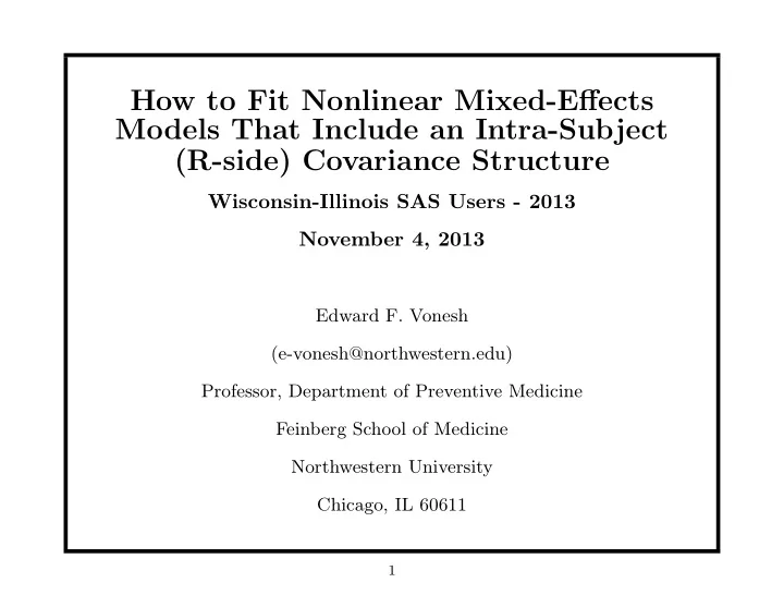
How to Fit Nonlinear Mixed-Effects Models That Include an Intra-Subject (R-side) Covariance Structure Wisconsin-Illinois SAS Users - 2013 November 4, 2013 Edward F. Vonesh (e-vonesh@northwestern.edu) Professor, Department of Preventive
How to Fit Nonlinear Mixed-Effects Models That Include an Intra-Subject (R-side) Covariance Structure Wisconsin-Illinois SAS Users - 2013 November 4, 2013 Edward F. Vonesh (e-vonesh@northwestern.edu) Professor, Department of Preventive Medicine Feinberg School of Medicine Northwestern University Chicago, IL 60611 1
Supplemental Material Much of the material including programs and data appear in the recently published book: Vonesh, Edward F. 2012. Generalized Linear and Nonlinear Models for Correlated Data: Theory and Applications Using SAS � . Cary, NC: SAS Institute Inc. Any examples taken directly from the book will be noted on the slides and likewise any corresponding material including datasets, programs, and SAS macros taken from the book can be found on the author’s web page: http://support.sas.com/publishing/authors/vonesh.html In some cases, the programs presented here have been modified slightly from those given in the book but the essential features remain the same. 2
Outline 1. Introduction . . . . . . . . . . . . . . . . . . . . . . . . . . . . . . . . . . . . . . . . . . . . . . . 4 2. Marginal and mixed models for correlated data . . . . . . 11 - Linear, generalized linear and generalized nonlinear models 3. Overview of estimation techniques in SAS . . . . . . . . . . . . 15 - GEE and MLE for marginal models - Conditional GEE (CGEE) and MLE for mixed models 4. Fitting nonlinear models in NLMIXED that include a within-subject (R-side) covariance structure . . . . . . . . . . . . . 18 - Example 1: Bone mineral density data - Example 2: Orange tree data 5. Conclusions . . . . . . . . . . . . . . . . . . . . . . . . . . . . . . . . . . . . . . . . . . . . . . . 68 3
1. Introduction Types of correlated data • Repeated measurements - data in which the response variable for each experimental unit is observed on multiple occasions and possibly under different experimental conditions. > Longitudinal data - data in which the underlying metameter (i.e., unit of measurement) for the occasions at which repeated measurements of the response variable are taken is time and interest generally centers on modeling trends over time. > Repeated measurements are more general in that the underlying metameter may be time or it may be a set of experimental conditions (e.g., dose levels of a drug). 4
Types of correlated data (continued) • Clustered data - data from experimental units are grouped into clusters resulting in within-cluster data that tend to be correlated > Correlation induced by clustering is more often than not accounted for through the specification of a random-effects model in which cluster-specific random effects are used to differentiate within- and between-cluster variability resulting in some form of intra-class correlation. > In some instances, there may be more than one level of clustering resulting in specification of a multi-level random-effects structure. For example, in a multi-center longitudinal trial, we may have a random center effect as well as repeated measurements on subjects within centers. 5
Types of correlated data (continued) • Spatially correlated data - data from studies where observations include both a response variable and a location vector associated with that response variable. The location vector describes the position or location at which the measured response was obtained. The proximity of measured responses with one another determines the extent to which they are correlated. > Lattice data , where measurements are linked to discrete regions (e.g., townships, counties, etc.) rather than some continuous coordinate system, are also considered as spatially correlated and are usually obtained from administrative data sources like census data, socio-economical data, and health data. 6
Types of covariates: • Within-unit factors or time-dependent covariates or repeated measures factors - Time itself - Different dose levels in a dose-response study - Different treatment levels in a crossover study • Between-unit factors or time-independent covariates - Baseline characteristics like gender, race, baseline age - Different treatment levels in a randomized prospective longitudinal study 7
Examples of repeated measurements: • Pharmacokinetic studies Clinical studies where the plasma concentration of a drug is measured at several time points for each subject • Panel data Econometric studies entailing both cross-sectional and time-series data together in a two-dimensional array. • Crossover studies (e.g., AB | BA) Clinical studies where each subject receives each treatment on possibly more than one occasion • Longitudinal studies Pediatric studies examining the growth pattern of children. Agricultural studies examining the growth pattern of plants. 8
Examples of clustered data: • Paired data Studies on twins where each pair serves as a natural cluster. Ophthalmology studies where a pair of eyes serves as a cluster. • Familial or teratologic studies Studies on members of a litter of animals (toxicology studies). Epidemiology studies of cancer where families serve as clusters. • Multi-center studies RCT’s where observations from subjects within a center (cluster) may be correlated (intra-class correlation). • Agricultural studies Studies in which different plots of land serve as clusters and measurements within a plot are homogeneous. 9
Examples of spatially correlated data: • Geostatistical data Forestry and agronomy studies where sampling from specified (fixed) locations is used to draw inference over an entire region accounting for spatial dependencies. • Epidemiological studies Studies aimed at describing the incidence and prevalence of a particular disease often rely on spatial correlation to explain regional variations associated with the disease. • Image analysis Image segmentation studies in the field of medicine are often used to help identify tissue regions that have been stained versus not stained. 10
2. Marginal and mixed models for correlated data Linear Models - Linear models (LM’s) - marginal - Linear mixed-effects (LME) models Generalized Linear Models - Generalized linear models (GLIM’s) - marginal - Generalized linear mixed-effects (GLME) models Generalized Nonlinear Models - Generalized nonlinear models (GNLM’s) - marginal > Normal-theory nonlinear model (NLM) - Generalized nonlinear mixed-effects (GNLME) models > Normal-theory nonlinear mixed-effects (NLME) model ◭ 11
Nonlinear mixed-effects (NLME) model The normal-theory nonlinear mixed-effects (NLME) model for correlated responses may be written as y ij = f ( x ′ ij , β , b i ) + w ij ( x ′ ij , β , b i ) − 1 / 2 ǫ ij , i = 1 , . . . , n ; j = 1 , . . . , p i where y ij is the j th measurement on the i th subject or cluster x ′ ij are 1 × u vectors of within- and between-subject covariates β is an s × 1 unknown vector of regression parameters b i are v × 1 vectors of random-effects ∼ iid N ( 0 , Ψ ( θ b )) w ij ( x ′ ij , β , b i ) are scalar weights that may depend on β and b i ǫ i = ( ǫ i 1 , ǫ i 2 , . . . , ǫ ip i ) ′ are p i × 1 random error vectors that are mutually independent and distributed as N p i ( 0 , Λ i ( θ w )) 12
Nonlinear mixed-effects (NLME) model We can write this model in matrix form as follows: y i = f ( X i , β , b i ) + W i ( X i , β , b i ) − 1 / 2 ǫ i , where y i is the p i × 1 response vector, y i = ( y i 1 . . . y ip i ) ′ X i is a p i × u design matrix of within- and between-subject covariates formed from the row vectors x ′ ij ǫ i ∼ ind N p i ( 0 , Λ i ( θ w )) W i ( X i , β , b i ) − 1 / 2 = Diag { w ij ( x ′ ij , β , b i ) − 1 / 2 } Let Λ i ( β , b i , θ w ) be the p i × p i covariance matrix of ( y i | b i ) where Λ i ( β , b i , θ w ) = W i ( X i , β , b i ) − 1 / 2 Λ i ( θ w ) W i ( X i , β , b i ) − 1 / 2 depends on a d w × 1 parameter vector θ w and possibly on β and b i . 13
Nonlinear mixed-effects (NLME) model Using the familar SAS notation from PROC MIXED, we have Λ i ( θ w ) is an R-side (within-subject) covariance matrix Ψ ( θ b ) is a G-side (random-effects) covariance matrix Problem: While SAS procedures MIXED and GLIMMIX allow for both an R-side and G-side covariance structure that includes directly specifying a within-subject correlation structure, the NLMIXED procedure does not currently support R-side covariance structures. The ǫ ij are assumed to be conditionally independent given b i 14
3. Overview of estimation techniques in SAS Estimation for marginal models (GLIM and GNLM) Generalized Estimating Equations (GEE) - GENMOD, GLIMMIX, %NLINMIX, NLMIXED Maximum Likelihood Estimation (MLE) - GLIMMIX, NLMIXED Estimation for mixed models (GLME and GNLME) Conditional Generalized Estimating Equations (CGEE) - GLIMMIX, %NLINMIX Maximum Likelihood Estimation (MLE) - GLIMMIX, NLMIXED 15
Estimation for mixed models (GLME, GNLME) Conditional GEE (CGEE) based estimation CGEE involves solving a set of first-order CGEE (CGEE1) for ( β , b 1 , . . . , b n ) and PL estimating equations for θ = ( θ b , θ w ). - Penalized nonlinear LS (PNLS) (Lindstrom and Bates, 1990) - Penalized quasi-likelihood (PQL) (Breslow and Clayton, 1993) - Pseudo-likelihood (PL) estimation (Wolfinger and Lin, 1993) This is the approach implemented in the SAS macro %NLINMIX for NLME models and an optional approach in the GLIMMIX procedure for GLME models 16
Recommend
More recommend
Explore More Topics
Stay informed with curated content and fresh updates.
