B-Splines as Finite Elements Ulrich Reif Darmstadt University of - PowerPoint PPT Presentation
1 B-Splines as Finite Elements Ulrich Reif Darmstadt University of Technology Joint work with K. K ollig, J. Wipper, and B. M oner WCCM, July 17, 2006 2 Splines: The d -variate B-splines of order n on the uniform grid h Z d are
1 B-Splines as Finite Elements Ulrich Reif Darmstadt University of Technology ❆ Joint work with K. K¨ ollig, J. Wipper, and B. M¨ oßner WCCM, July 17, 2006
2 Splines: The d -variate B-splines of order n on the uniform grid h Z d are denoted b n k , k ∈ Z d . x 2 k 2 h kh 0 k 1 h x 1 If the domain is restricted to Ω ⊂ R d , use only B n := { b n k : supp b n k ∩ Ω � = ∅} . A spline is a linear combination of B-splines with control points, � b n k p k = B n P. s = k
3 Main features: ❏ high approximation order, � u − s h � = O ( h n ) ❏ few dof (one per grid cell) ❏ mesh generation is trivial ❏ local support yields small band widths ❏ local refinement ❏ efficient algorithms and data structures
3 Main features: ❏ high approximation order, � u − s h � = O ( h n ) ❏ few dof (one per grid cell) ❏ mesh generation is trivial ❏ local support yields small band widths ❏ local refinement ❏ efficient algorithms and data structures Why are B-splines not commonly used for FE-approximations?
4 Problems: ❏ Boundary conditions: If a spline is forced to be zero at the boundary of Ω , then it vanishes on all intersecting grid cells (in general). This implies a complete loss of approximation power. ❏ Condition number: B-splines with small support in Ω may lead to excessively large condition numbers. Leaving out outer B-splines reduces approximation power.
5 Extension: Partition the set K of relevant indices as follows: The inner B-splines with indices The outer B-splines with indices I ⊂ K J = K \ I have at least one grid cell in have no grid cell in their support their support contained in Ω . contained in Ω .
6 Extension: In order to stabilize the basis, the outer B-splines are no longer considered to be independent, but coupled with inner B-splines, � i ∈ I. B i = b i + e i,j b j , j ∈ J
7 Extension: Choose coefficients e i,j in such a way that all polynomials of order n remain in the span of the B i using Marsden’s identity, � p ( k ) b k ∈ I p ∈ I P n (Ω) iff P n ( K ) . k ∈ K and Lagrange interpolation of neighboring inner control points. 3 −3 1 0 0 0 0 0 0 0 1 3 0 0 3
8 Weighting: The incorporation of zero boundary conditions is amazingly simple. Let w : Ω → R + 0 be a smooth function equivalent to the boundary distance, i.e. w ( x ) dist( x, ∂ Ω) dist( x, ∂ Ω) � 1 , � 1 , w ( x ) and in particular w = 0 exactly on ∂ Ω . Multiplying the extended B-splines B i by the weight function w yields a basis which satisfies the boundary condition.
9 Definition: The weighted extended B-splines B i (web-splines) are defined by w � � � i ∈ I, B i = b i + e i,j b j , w ( x i ) j ∈ J ( i ) where x ( i ) is the center of a grid cell in supp b i ∩ Ω . The web-splines span the web-space I B := span { B i : i ∈ I } .
10 Theorem: The web-basis has essentially the same stability properties as the standard B-splines basis, � � � � r � h − r � A � . � � 0 ∼ � A � , a i B i a i B i � � � � � � � � i ∈ I i ∈ I
10 Theorem: The web-basis has essentially the same stability properties as the standard B-splines basis, � � � � r � h − r � A � . � � 0 ∼ � A � , a i B i a i B i � � � � � � � � i ∈ I i ∈ I Theorem: The condition number of the Galerkin matrix is bounded by cond G h � h − 2 .
10 Theorem: The web-basis has essentially the same stability properties as the standard B-splines basis, � � � � r � h − r � A � . � � 0 ∼ � A � , a i B i a i B i � � � � � � � � i ∈ I i ∈ I Theorem: The condition number of the Galerkin matrix is bounded by cond G h � h − 2 . Theorem: web-splines have essentially the same (optimal) approximation properties as standard B-splines. More precisely, for 0 ∩ H k there exists a web-spline s h such that for all k ≤ n u ∈ H 1 � u − s h � r � � u � k h k − r .
11 Example 1: Helmholtz equation Compute many (several thousand) eigenvalues of the Laplacian in order to understand quantum mechanics of small particles, ∆ u + λu = 0 in Ω , u = 0 on ∂ Ω .
11 Example 1: Helmholtz equation Compute many (several thousand) eigenvalues of the Laplacian in order to understand quantum mechanics of small particles, ∆ u + λu = 0 in Ω , u = 0 on ∂ Ω .
12 The FE-discretization leads to a generalized eigenvalue problem, Av = λBv. # EV CPU time (h) standard technique 200 100
12 The FE-discretization leads to a generalized eigenvalue problem, Av = λBv. # EV CPU time (h) standard technique 200 100 multigrid 2000 100
12 The FE-discretization leads to a generalized eigenvalue problem, Av = λBv. # EV CPU time (h) standard technique 200 100 multigrid 2000 100 web-splines 2000 1
13
14
15
16
17
18
19 Example 2: Reverse engineering Given: Data points ( x i , y i , z i ) sampled on domain Ω from function f . Sought: Function g : Ω → R with g ( x i , y i ) ≈ z i . 3 2 1 0 −1 −2 −3 −4 −2 0 2 4
20 standard B-splines ℓ ∞ -error: 2 . 1 e- 4 L ∞ -error: 2 . 8 e- 1 condition number 6 . 2 e+ 13
20 standard B-splines extended B-splines ℓ ∞ -error: 2 . 1 e- 4 ℓ ∞ -error: 2 . 2 e- 4 L ∞ -error: 2 . 8 e- 1 L ∞ -error: 2 . 3 e- 4 condition number 6 . 2 e+ 13 condition number 7 . 7 e+ 3
21 Stabilization by normalization: f ( x ) = b i ( x )
22 Stabilization by normalization: B i ( x ) := b i ( x ) � b i � ∞
23 Stabilization in 1d stable stable not stable
23 Stabilization in 1d stable stable not stable Stabilization in 2d stable stable not stable (rare)
24 Definition: A normalized B-Spline B i is called p -stable on Ω ⊂ R d , if there exist intervals Q ⊂ P ⊂ supp b i such that ❏ Q ⊂ Ω is contained in a grid cell ❏ P and supp b i have a common corner ❏ n [ Q ] = [ P ] ❏ � b i � p, Ω ≤ � b i � p,P The index set of p -stable B-splines is denoted I p . Theorem The basis { B i : i ∈ I p } is stable with respect to the p -norm. The constants depend only on n and p . Further, this basis provides full approximation power wrt. the L 2 -norm.
25 Current work: Stokes equation − ∆ u + ∇ p = in Ω f div u = 0 in Ω = 0 on ∂ Ω u Conjecture: The Babuˇ ska-Brezzi-condition � inf sup p div u ≥ β > 0 p ∈ P u ∈ U Ω � p � 0=1 � u � 1=1 is satisfied for � ( n + 1) × n � deg P = n × n, deg U = . n × ( n + 1)
26 Conclusion: ❏ web-splines • form a stable basis • have full approximation power • are well suited for FE-simulations and reverse engineering
26 Conclusion: ❏ web-splines • form a stable basis • have full approximation power • are well suited for FE-simulations and reverse engineering ❏ selected normalized B-splines • form a stable basis • have full approximation power (under mild assumptions) • are well suited for FE-simulations
26 Conclusion: ❏ web-splines • form a stable basis • have full approximation power • are well suited for FE-simulations and reverse engineering ❏ selected normalized B-splines • form a stable basis • have full approximation power (under mild assumptions) • are well suited for FE-simulations For further information, visit www.web-spline.de
27 1 0.5 0 −0.5 −1 −1 −0.5 0 0.5 1
28 −0.5 −0.5
29
30
Recommend
More recommend
Explore More Topics
Stay informed with curated content and fresh updates.
