Paper Summaries Any takers? Interpolation Projects Factoids - PDF document
Paper Summaries Any takers? Interpolation Projects Factoids Proposals due next week. Digital Video Frame Rate Star Wars was shot at 24 fps. Keep film look Plan for today Motivation Films Keyframing and
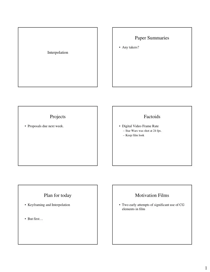
Paper Summaries • Any takers? Interpolation Projects Factoids • Proposals due next week. • Digital Video Frame Rate – Star Wars was shot at 24 fps. – Keep film look Plan for today Motivation Films • Keyframing and Interpolation • Two early attempts of significant use of CG elements in film • But first… 1
Motivational Film Motivational Film • TRON • Question from SIGGRAPH Bowl – Disney (1982) – Q: Which special effects company was responsible for the effects of TRON? – Clips shown at SIGGRAPH 82 – A: ALL OF THEM • MAGI • Triple I • Robert Abel & Associates • Digital Effects Motivational Film Motivational Film • Interesting TRON Factoid • The Last Starfighter (1985) – No polygons! – Effects by Digital Productions – All objects were defined using mathematical – Universal Pictures formula. • Lesson Learned from TRON – Great effects – Bad movie – Overestimated the “Geek Factor” Motivational Film Motivational Film • Last Starfighter factoids • Life imitating art imitating life… – First movie to do all special effects (except makeup) on – Sort of… a computer. – A prototype for A Last Starfighter video game – All shots of spacecraft, space, etc. were generated on a was produced by Atari (remember them?) but Cray computer. was never distributed. • Lesson Learned from Last Starfighter – Note that there WAS a TRON video game – Great effects (made by Bally/Midway – 1983) – Bad movie – Overestimated the “Geek Factor” 2
Let’s get started 6. Straight ahead action and Pose-to-pose action • Key framing and interpolation • The two main approaches to hand drawn animation. – Straight ahead action • “the animator works straight ahead from his first drawing in the scene.” – Pose-to-pose (keyframing) • the animator plans his actions, figures out just what drawings will be needed to animate the business, makes the drawings concentrating on the poses, ... and then draws the inbetweens.” • Link Key framing Key Framing • The simplest form of animating an object. P 4 • Object has: P 2 P 5 – A beginning state Time = 50 Time = 10 – An end state Time = 55 P 1 – A number of intermediate “key” states P 6 P 3 • It is up to the keyframe system to determine Time = 0 the states for inbetween frames Time = 60 Time = 35 Key Framing Interpolation • 60 sec animation • According to webster.com – Video: 30 frames / sec = 1800 frames – in·ter·po·late (n) - to estimate values of (a function) between two known values – We have 6 key frames – Need to create position of objects for the remaining 1794 frames. – Note: “state” can be defined as a function (in this case of time) • F(t) 3
Interpolation Interpolation • Things to consider: • Things to consider: – Interpolation or approximation? – Continuity – defines “smoothness” of curve. • Interpolation – Control points fall on the curve – Determined by how many derivatives are • Approximation – Control points fall outside the continuous curve. • 0 th order – are the curves attached at the points themselves (positional continuity) • 1 st order – is the first derivative continuous (tangential continuity) • 2 nd order – is the 2 nd derivative continuous (curvature continuity) Interpolation – Continuity Interpolation • Things to consider: – Local vs. Global control • Does changing one point change the entire function? No positional Order 0 2 nd order Order 1 continuity continuity Continuity continuity – Questions? For animation purposes, Tangential (1 st Order) continuity is usually sufficient Linear Interpolation Linear Interpolation • The simplest solution • Pros – Straight-forward = − ⋅ + ⋅ P ( u ) ( 1 u ) P u P 0 1 – Easy to implement P(t) P(1) = P 1 Also can be – Direct relationship between time and value expressed as • Cons = − ⋅ + P ( u ) ( P P ) u P – Lacks tangential continuity 1 0 0 P(0) = P 0 – Why is this important? 4
Cubic Interpolation Remember our principles of animation? • 8. Arcs • x, y, z given as function of t – “The visual path of action from one extreme to • Approximated by cubic polynomials another is always described by an arc.” = + + + 3 2 x ( t ) a t b t c t d x x x x = + + + 3 2 y ( t ) a t b t c t d y y y y = + + + 3 2 z ( t ) a t b t c t d z z z z This is not an arc! Cubic Interpolation Cubic Interpolation • Separate C matrix into basis + geometry ⎡ ⎤ a a a y x z ⎢ ⎥ b [ ] b b ⎢ ⎥ = ⎡ ⎤ ⎡ ⎤ = y Q ( t ) x ( t ) y ( t ) z ( t ) x z G m m m m G G C 1 y ⎢ ⎥ 11 12 13 14 1 x 1 z ⎢ ⎥ ⎢ ⎥ c c c m m m m G G G ⎢ ⎥ ⎢ y ⎥ ⎢ ⎥ [ ] x z = 2 y 21 22 23 24 2 x 2 z C T = 3 2 ⎢ ⎥ ⎢ ⎥ ⎢ ⎥ t t t 1 d ⎣ d d ⎦ G m m m m G G y 3 y x z 31 32 33 34 ⎢ 3 x 3 z ⎥ ⎢ ⎥ ⎢ ⎥ ⎣ m m m m ⎦ ⎣ G G G ⎦ = ⋅ 1 4 4 4 4 2 4 4 4 4 3 4 y 41 42 43 44 1 4 2 4 4 x 4 3 4 4 z Q T C basis matrix control points Cubic Interpolation Cubic Interpolation • Hermite Curves = ⋅ ⋅ – specified by endpoints and tangent vectors from Q ( t ) T M G { { each endpoint basis control • Basis & Control points distinguishes types of curves 5
Cubic Interpolation Cubic Interpolation • Hermite Curves • Problem with Hermite Curves – Animator generally will not enjoy specifying ⎡ − ⎤ ⎡ ⎤ 2 2 1 1 P 1 tangent vectors ⎢ ⎥ ⎢ ⎥ − − − 3 3 2 1 ⎢ ⎥ P ⎢ ⎥ = = 4 M G H ⎢ ⎥ ⎢ ⎥ H 0 0 1 0 R ⎢ ⎥ 1 ⎢ ⎥ – Solution: The Catmull-Rom spline ⎣ 1 0 0 0 ⎦ ⎣ R ⎦ 4 Cubic Interpolation Cubic Interpolation • Catmull-Rom spline • Catmull-Rom – Uses previous and next control point to determine − − ⎡ ⎤ ⎡ ⎤ 1 3 3 1 P tangent vector − i 1 ⎢ ⎥ ⎢ ⎥ − − 2 5 4 1 1 P ⎢ ⎥ ⎢ ⎥ = = i M G ⎢ − ⎥ CR ⎢ ⎥ CR 2 1 0 1 0 P + ⎢ ⎥ ⎢ i 1 ⎥ ⎣ ⎦ 0 2 0 0 ⎣ P ⎦ + i 2 Note: for interpolation between P i and P i+1 you need 4 points – Spline goes through all control points! Cubic Interpolation Cubic Interpolation • Bezier Curves • Bezier Curves – specified by endpoints and intermediate points, − − ⎡ ⎤ ⎡ ⎤ 1 3 3 1 P not on the curve, that approximate the tangent ⎢ ⎥ 0 ⎢ ⎥ − − vectors 3 6 3 0 P ⎢ ⎥ ⎢ ⎥ = = 1 M G H ⎢ ⎥ B − ⎢ ⎥ 3 3 0 0 P ⎢ ⎥ 2 ⎢ ⎥ ⎣ ⎦ 1 0 0 0 ⎣ ⎦ P 3 6
Cubic Interpolation Cubic Interpolation • Bezier Curves suffer from same problem as • B-Splines Hermite Curves – Control points are outside of the curve – Animator generally will not enjoy specifying tangent – Local control vectors…even from control points • Moving one control point only affects a portion of • Exception: Provide animator with an interactive curve editor the entire curve. – DeCastelau Construction – Individual curve segments share control points. • Algorithm to automatically define Bezier control points • Described in Parent Appendix and Shomake Quat. paper – Knots - points connecting individual curve segments. Cubic Interpolation Cubic Interpolation • B-Splines • B-Splines - local control Cubic Interpolation Cubic Interpolation • Segment Q i uses control points P i-3 , P i-2 , P i-1 and P i • B-Splines − − ⎡ ⎤ ⎡ ⎤ 1 3 3 1 P − i 3 ⎢ ⎥ ⎢ ⎥ − − 3 6 3 0 1 P ⎢ ⎥ ⎢ ⎥ = = − i 2 M G ⎢ ⎥ B − ⎢ ⎥ H 6 3 0 3 0 P − ⎢ ⎥ ⎢ i 1 ⎥ ⎣ ⎦ 1 4 1 0 ⎣ ⎦ P i 7
Cubic Interpolation Cubic Interpolation • Rational Splines • Uniform Nonrational B-Splines – expressed using homogeneous coordinates – uniform - knots are equally spaced [ ] = – nonrational - does not use homogeneous Q ( t ) X ( t ) Y ( t ) Z ( t ) W ( t ) coordinates (more on this later) – B - basis -- curves are weighted sums of a basis X ( t ) Y ( t ) Z ( t ) = = = function x ( t ) , y ( t ) , z ( t ) W ( t ) W ( t ) W ( t ) Cubic Interpolation Cubic Interpolation • Rational splines -- why bother? • NURBS – Invariant under rotation, scaling, translation, – Non-uniform Rational B-Splines and perspective transforms – Non-uniform - knots need not be equally – Can define precisely any of the conic sections. spaced. (spheres, ellipsoids, parabolids, etc) – Most useful and used method for representing surface curves in CG. – Probably overkill for cubic interpolation Cubic Interpolation Cubic Splines • Pros – We now have our tangential continuity u=0.0 – More complex than linear but not too complex • Cons u=2/3 – Spline control does not correspond to time. u=1.0 u=1/3 – May require an interactive “curve editor” tool. u does not correspond to t. 8
Recommend
More recommend
Explore More Topics
Stay informed with curated content and fresh updates.
