Fast Direct Methods for Gaussian Processes Mike ONeil Departments - PowerPoint PPT Presentation
Fast Direct Methods for Gaussian Processes Mike ONeil Departments of Mathematics New York University oneil@cims.nyu.edu December 12, 2015 1 Collaborators This is joint work with: Siva Ambikasaran (ICTS, Tata Institute) Dan
Fast Direct Methods for Gaussian Processes Mike O’Neil Departments of Mathematics New York University oneil@cims.nyu.edu December 12, 2015 1
Collaborators This is joint work with: Siva Ambikasaran (ICTS, Tata Institute) Dan Foreman-Mackey (UW Astronomy) Leslie Greengard (NYU Math, Simons Fnd.) David Hogg (NYU Physics) Sunli Tang (NYU Math) 2
The short story: Results I will present a fast, direct (not iterative), algorithm for rapidly evaluating likelihood functions of the form: 1 (det C ) 1 / 2 e − y t C − 1 y L ( θ ) θ ) ∝ These likelihood functions universally occur when modeling under Gaussian process priors. 3
Outline • Probability review • Gaussian process overview • Applications: Regression & prediction • Computational bottlenecks • A fast algorithm • Numerical results • Other and future work 4
Multivariate normal The n-dimensional normal distribution has the following properties: 1 Z µ ) t C − 1 ( ~ P ( ~ (2 ⇡ ) n/ 2 | det C | 1 / 2 e − ( ~ y − ~ y − ~ µ ) / 2 d ~ X ∈ ! ) = y ! C is a positive-definite covariance matrix C ij = Cov ( X i , X j ) 5
Stochastic processes Stochastic processes are simply the generalization of random variables to random functions 6
Gaussian processes are stochastic processes 7
Gaussian processes Random functions with structured covariance 8
Gaussian processes We say that f ( x ) ∼ GP ( m ( x ) , k ( x, x 0 )) if and only if f ( x 1 ) , . . . , f ( x n ) ∼ N ( m ( x ) , C ) m = ( m ( x 1 ) · · · m ( x n )) t C ij = k ( x i , x j ) The function k is the covariance kernel 9
Gaussian processes This means that each realization of a Gaussian process is a function - the corresponding probability distribution is over functions . This function sampled at a selection of points behaves like a multivariate Normal distribution Each marginal distribution is normal: f ( x i ) ∼ N ( m ( x i ) , C ii ) 10
Role of the covariance kernel Admissible covariance kernels must give rise to positive-definite covariance matrices: y t K ( x , x ) y > 0 for all choices of x , y . Common choices are: k ( x, x 0 ) = e � | x � x 0 | /a k ( x, x 0 ) = e � ( x � x 0 ) 2 /b ✓ √ ◆ ν ✓ | x − x 0 | 2 ν | x − x 0 | ◆ k ( x, x 0 ) = K ν c c 11
Many options for the covariance kernel 1.0 0.8 0.6 1.0 0.4 0.8 0.2 0.6 - 4 - 2 2 4 0.4 0.2 Figure 10.26.4 : K ν ( x ), 0 . 1 ≤ x ≤ 5 , 0 ≤ ν ≤ 4. - 4 - 2 2 4 (c) Nist Handbook 8 1.0 6 0.5 4 2 - 4 - 2 2 4 - 6 - 4 - 2 2 4 6 - 0.5 12
Role of the covariance kernel The covariance kernel controls the regularity and the variability of the Gaussian process. k ( x, x 0 ) = e � ( x � x 0 ) 2 / (20) k ( x, x 0 ) = e � ( x � x 0 ) 2 / (0 . 2) (95% Conditional confidence intervals are shaded) 13
GP ’s in action: Prediction Imagine we have data { x , y }, and assume a model of the form: y i = f ( x i ) + ✏ i Furthermore, assume that f is a Gaussian process and that is i.i.d. Gaussian noise ( priors ): ✏ i f ∼ GP ( m θ , k θ ) ✏ ∼ N (0 , � 2 ) We’ve assumed that f can depend on some other set of parameters, which we may fit later. θ 14
Prediction This implies that y is also a Gaussian process : y ( x ) ∼ GP ( m θ ( x ) , δ ( x − x 0 ) σ 2 + k θ ( x, x 0 )) The new covariance matrix is: C = σ 2 I + K θ 15
Prediction Assume m ( x) = 0 . Then the joint distribution of y and a new predicted value is: y ∗ y � ✓ �◆ k ( x , x ∗ ) C ∼ N 0 , k ( x ∗ , x ) k ( x ∗ , x ∗ ) y ∗ 16
Prediction The conditional distribution (posterior) of the predicted value can then be calculated as: y ∗ | x , y , x ∗ ∼ N ( µ, η 2 ) where µ = k ( x ∗ , x ) C − 1 y η 2 = k ( x ∗ , x ∗ ) − k ( x ∗ , x ) C − 1 k ( x , x ∗ ) Schur complement of C 17
What about the extra parameters? k = k ( x, x 0 ; θ 1 ) In general, m = m ( x ; θ 2 ) The parameters have to be fit to the data (inference), or marginalized away (integrated out). 18
Computational bottlenecks There are three main computational bottlenecks in dealing with large covariance matrices: C − 1 • Computation/application of • Computation of log det C C = W t W • Symmetric factorization e − y t C − 1 θ ( x ) y / 2 L ( θ ) = (2 π ) n/ 2 | det C θ ( x ) | 1 / 2 19
Alternative existing methods To avoid large-scale dense linear algebra, various techniques are often used to approximate the inverse and determinant: • Element thresholding (banded/sparse matrix) • Special-case kernels (exponential) • Subsampling • Iterative methods In many cases, these methods sacrifice the fidelity of the underlying model. 20
Hierarchical matrix compression We want a data-sparse factorization of the covariance matrix which allows for fast inversion: A = A 1 A 2 · · · A m means that A − 1 = A − 1 m A − 1 m − 1 · · · A − 1 1 det A = det A 1 det A 2 · · · det A m Many factorizations can be used: HODLR, HBS, HSS, etc. 21
Hierarchical matrix compression What properties of the Gaussian process covariance matrix allow for it to be rapidly factored? For example, most covariance kernels yield matrices which are Hierarchically Off-Diagonal Low-Rank Full rank; Low rank; 22
Hierarchical matrix compression The resulting (numerical) factorization will have the form: × × × = K (3) K 3 K 2 K 1 K 0 Full rank; Low-rank; Identity matrix; Zero matrix; Physical interpretation? 23
Motivation: Physics F = − G m 1 m 2 r 2 24
Motivation: Physics Calculations required: O ( N ) (In FINITE arithmetic) Fast Multipole Methods F = − G m 1 m 2 r 2 25
Motivation: Physics Similar algorithms exist for Heat Flow , where the distribution looks like a Gaussian: 1.0 0.8 Temperature 0.6 0.4 0.2 - 4 - 2 2 4 Distance 26
Connection with statistics Time series data which occurs close in time has larger relationship than data occurring far apart . 1.0 0.8 Temperature 0.6 Often this covariance is modeled 0.4 using the heat kernel : 0.2 - 4 - 2 2 4 Distance 27
A 1-level scheme - in pictures We can easily show how the factorization works for a 1-level scheme: = x Full rank; Low-rank; Identity matrix; Zero matrix; 28
A 1-level scheme - in formulae We can easily show how the factorization works for a 1-level scheme: UV t A 11 A 11 I 0 A − 1 11 UV t = x A 22 V U t A 22 A − 1 I 0 22 V U t Assume we have the factors U and V for now. 29
A 2-level scheme - in formulae A 2-level factorization is slightly more complicated… I U 1 V t 0 A 11 A 11 A − 1 11 U 1 V t 1 1 UV t I 0 0 A − 1 1 UV t I 0 A 22 V 1 U t A 22 A − 1 22 V 1 U t 1 1 = x x I I A 33 0 A − 1 33 U 2 V t U 2 V t A 33 2 2 V U t I 0 0 A − 1 2 V U t I 0 V 2 U t A 44 A 44 A − 1 44 V 2 U t 2 2 A 11 U 1 V t A 33 U 2 V t 1 2 where A 1 = and = A 2 V 1 U t A 22 V 2 U t A 44 2 1 30
A 2-level scheme - in formulae U 1 V t A 11 1 How do we invert = A 1 ? A 22 V 1 U t 1 � 0 A 11 � U 1 � V t 0 0 1 = + U t A 22 V 1 0 0 0 1 We can use the Sherman-Morrison-Woodbury formula: � − 1 V A − 1 ( A + UV ) − 1 = A − 1 − A − 1 U I + V A − 1 U � If U,V are rank k , this is a k x k matrix 31
A log( n )-level scheme Proceeding recursively… × × × = K (3) K 3 K 2 K 1 K 0 Full rank; Low-rank; Identity matrix; Zero matrix; 32
Low-rank factorizations Two classes of techniques: • Linear algebraic • SVD, LU, LSR, etc. • Analytic • Explicit outer product O ( n 2 k ) Most linear algebraic dense methods scale as . Analytic (polynomial) interpolation of the kernel can O ( nk 2 ) scale as . Special function expansions may be fastest. 33
Analytic approximation For example, the squared-exponential (Gaussian) function can be written as: ✓ s ✓ t ◆ n ∞ ◆ 1 e − ( t − s ) 2 / ` = e − t 2 / ` X H n √ √ n ! ` ` n =0 Similar (approximate) expansions can be calculated for most kernels in terms of other special functions. 34
Analytic approximation Matérn kernels: ◆ ν ✓ √ ✓ √ k ( r ) = 2 1 − ν 2 ⌫ r 2 ⌫ r ◆ K ν Γ ( ⌫ ) ` ` Bessel functions obey the addition formula: ∞ ( − 1) j K ν + j ( w ) I j ( z ) X K ν ( w − z ) = j = −∞ 35
High-order interpolation When given a form of the covariance kernel, we have the ability to evaluate it anywhere , including at locations other than those supplied in the data: p p X X K ( x, y ) ≈ K ( x i , y j ) L j ( x ) L k ( y ) i =1 j =1 Choose interpolation nodes to be Chebyshev nodes for stable evaluation, and formulaic factorizations. 36
Computational complexity Using ACA (LU) with randomized accuracy checking or O ( np 2 ) Chebyshev interpolation, we can factor A = UV in time, p is the numerical rank. O ( np 2 ) Compute all low-rank factorizations: On level k , we have to update k other U blocks: O ( knp 2 ) log n O ( kp 2 n ) = O ( p 2 n log 2 n ) X k =1 Inversion and determinant are both: O ( p 2 n log n ) 37
Recommend
More recommend
Explore More Topics
Stay informed with curated content and fresh updates.
