Exploring the z~2-3 Cosmic web with 3D Lyman-alpha Forest absorption - PowerPoint PPT Presentation
Exploring the z~2-3 Cosmic web with 3D Lyman-alpha Forest absorption tomography Sakura CLAW @ University of Tokyo March 28, 2018 Khee-Gan (K.-G,) Lee Kavli IPMU, Kashiwa, Japan @kheegster, #27393124 Collaborators: Alex
Exploring the z~2-3 Cosmic web with 3D Lyman-alpha Forest absorption tomography Sakura CLAW @ University of Tokyo March 28, 2018 Khee-Gan (“K.-G,”) Lee Kavli IPMU, Kashiwa, Japan @kheegster, #27393124 Collaborators: Alex Krolewski (Berkeley grad student), Martin White (Berkeley), David Schlegel (LBNL),, Xavier Prochaska (UCSC), Joe Hennawi (UCSB), John Silverman (IPMU), Nao Suzuki (IPMU), Masami Ouchi (UTokyo), Peter Nugent (LBNL), Zarija Lukic (LBNL) 1
http://ipmu.jp/igm2018 2
The Lyman-alpha Forest Absorption at z>2 Restframe 1215.67Å absorption from neutral HI in intergalactic medium 3
Fluctuating Gunn-Peterson Approximation (FGPA) • Current paradigm for large-scale IGM: ~uniform optically-thin photo-ionization (ignoring DLAs etc) • Lyman-alpha forest optical depth is modulated by IGM astrophysics and underlying large-scale structure overdensity • Optical depth is modulated by uniform UV background levels 𝛥 bg , IGM temperature T 0 , slope of temperature-density relationship 𝛿 Credit: Rob Simcoe In this talk, I assume We observe transmitted flux, F=F 0 exp(- 𝜐 ) (absorption traces large-scale structure) 4
IGM Tomography: Mapping 3D Ly-alpha forest • If have a grid of closely-separated sightlines, could allow reconstruction of 3D absorption field on scales comparable to sightline separation ( Pichon+2001, Caucci+2008, Lee +2014 ) Credit: Casey Stark (UC Berkeley) Going fainter → More sightlines → Smaller scales 5
GOING BEYOND QUASARS FOR LY -ALPHA FOREST Average sightline separation # of Ly-a forest sightlines per sq deg 25/deg 2 10/deg 2 Huge jump in sightline availability BOSS DESI with LBGs/star-forming galaxies! (2.5m) (4m)
Sources Within A 12’x12’ Field mag<22.5 QSOs at 2.3<z<3.0 7
Sources Within A 12’x12’ Field mag<24.5 QSOs+Galaxies at 2.3<z<3.0 8
COSMOS LYMAN-ALPHA MAPPING AND TOMOGRAPHY OBSERVATIONS (CLAMATO) • Keck survey on COSMOS field (10hr, +02deg) • Aim to get spectra LBGs+QSOs at z~2-3, to sample 2.1<z<2.5 Ly-a forest with sightline separations of ~2.5h -1 Mpc • First systematic use of galaxies as Ly 𝛽 forest background sources • 2-4hr integrations with Keck-I/LRIS spectrograph down to g<24.8 • ~60hrs on-sky observations so far
Current Status: 230 sightlines over 27’ × 21’ area (0.17 deg 2 ), covering 2.05<z<2.55 with mean transverse separation d ⊥ =2.4h -1 Mpc 30 h -1 Mpc COSMOS/CANDELS Field 24 h -1 Mpc 10
Ly 𝛽 of background source Ly 𝛽 forest Ly 𝛽 forest Ly 𝛽 forest Color scheme: spectrum , noise vector, spectral template
Wiener Filtering Of Sightlines • We have the flux 𝜀 F , pixel noise, and their [x,y,z] positions. Estimate map, M , using Wiener filter applied to data D and noise matrix N • Assume a correlation matrix of the form C DD =C MD =C(r 1 ,r 2 ) • L || =2.5h -1 Mpc and L ⊥ =2.0h -1 Mpc are set by the sightline separation and resolution, 𝜏 F =0.8 is the variance of the map 12
CLAMATO IGM Survey at z~2.3 (Keck-I) Overdense Underdense Lee et al, 2017 DEEP2 Redshift Survey at z~1 (Keck-II) Coil et al, 2004 13
YouTube: http://tinyurl.com/clamatovid-v2 14
Come see the VR version at Alex Krolewski’s poster! 15
First Detection Of Cosmic Voids At High-z Krolewski, KGL, et al 2017, arXiv:1710.02612 24Mpc/h along Dec redshift • Most distant-known cosmic voids from galaxy redshift surveys are at z~0.9 (VIPERS Survey, Hawken+2016) • Clearly see coherent underdensities in the CLAMATO map at 2.05<z<2.55 • Search for voids in CLAMATO using simple “spherical underdensity” void finder (e.g. Stark, Font-Ribera, White, KGL, 2015) • Voids identified in the tomographic map are ~6 𝜏 underdense in spectroscopic galaxies • See poster by Alex Krolewski outside!
A forming supercluster at z=2.51? redshift y (Mpc/h) z (Mpc/h) • Known galaxy protoclusters at z=2.44 (Diener+2015, Chiang+2015), z=2.48 (Casey+2016) and z=2.51 (Wang+2016) are <100 cMpc from each other. • CLAMATO is resolving real filamentary sub-structure at z~2.5! 17
Inferring Map Initial Conditions “True” Initial Conditions Toy “observations” at z~2.5 Simple log-normal model for Ly-a • forest flux as function of density Limited-memory Broyden- • Fletcher-Goldfarb-Shanno (L- BFGS) algorithm to minimize likelihood Inferred initial conditions (z= ∞ ) • Inferred Initial Conditions Inferred velocities at z~2.5 can be used as a seed to run a sim to z=0 to infer fate of structures observed at z~2.5 with tomography Lead by B. Horowitz (UCB) and • M. White(UCB) 18
Galaxy-Forest Cross-Clustering • Cross-correlate CLAMATO forest pixels with spectroscopic surveys in COSMOS field (with Andreu Font-Ribera, UCL) • ~1500 galaxies at 2.0<z<2.6 within <15 Mpc/h transverse distance of at least 1 sightline, from zCOSMOS, VUDS, MOSDEF, ZFIRE, CLAMATO, 3D-HST • Objective: assume that forest bias and beta is known to derive galaxy free parameters Current CLAMATO 𝞀 Footprint 𝜀 F , n o i t p r o s b A Foreground 𝞃 galaxy Ly-a forest bias + RSD (known) Linear theory power spectrum Cross-power spectrum Galaxy bias + RSD (known from cosmology)
Preliminary! Cross-correlation with Galaxies Use simple inverse variance • estimator in configuration space (Font-Ribera et al 2012): Line-of-sight Overall ~21 𝞃 detection from all • samples Current analysis assumes forest bias • is fixed (known to ~3% from BOSS) Model galaxies with linear model. • with free parameters: bias, b • LOS offset, 𝜀 z • LOS dispersion, 𝞃 z (combination • Lee, Font-Ribera et al., in prep. of redshift error + FoG) Transverse
Studying The High-Z Cosmic Web With IGM Tomography Matter Density Mock CLAMATO • Lee & White 2016, ApJ, 817,160 δ F ∆ 100 100 4.00 0.17 0.13 3.50 80 80 0.09 3.00 • Krolewski, Lee , Lukic & White 2017, ApJ, 0.05 y (Mpc/h) 2.50 60 60 0.01 2.00 837,31 -0.03 40 40 1.50 -0.07 1.00 -0.11 20 20 0.50 -0.14 • Zel’dovich-like approach: eigenvalue analysis of 0 0.00 0 -0.18 0 20 40 60 80 100 0 20 40 60 80 100 the gravitational tidal tensor d 2 𝛸 /dx i dx j Dark matter cosmic web CLAMATO cosmic web 3.20 3.20 100 100 2.80 2.80 80 80 2.40 2.40 • tl;dr: IGM tomography provide good recovery y (Mpc/h) 2.00 2.00 60 60 the eigenvectors of the DM cosmic web 1.60 1.60 40 40 1.20 1.20 0.80 0.80 20 20 0.40 0.40 • With sufficient data volume, can constrain 0.00 0.00 0 0 0 20 40 60 80 100 0 20 40 60 80 100 intrinsic alignments from galaxies at Cosmic x (Mpc/h) x (Mpc/h) Noon 21
Future Surveys: Subaru-Prime Focus Spectrograph • Simultaneously observe ~2000 targets over 1.3deg^2 FOV (c.f. Keck-LRIS: ~20 objects over 0.01deg^2) • Broadband wavelength coverage: 380nm-1.3 micron • Proposed Subaru Strategic Program (SSP) proposal for ~300 nights covering: • Cosmology • Galactic Archeology • Galaxy Evolution • Projected to begin survey operations in 2021 22
IGM Tomography in PFS Galaxy Evolution Survey • 50 nights of the survey will be targeted at 2<z<7 universe • Area: 3 × 5 deg 2 • 970/deg 2 background sources at 2.5<z<3.5 (g<24.7) • 1000/deg 2 of foreground sources at 2.2<z<2.6 for cross-correlation CLAMATO (2017) Underdense Overdense Subaru-PFS Footprint 23
IGM Tomography with Keck vs PFS Subaru-PFS Galaxy CLAMATO (Keck-I/LRIS) Evolution SSP Area 0.16 deg 2 (in 2017) 15 deg 2 Map Volume 9 × 10 5 cMpc 3 4.4 × 10 7 cMpc 3 Background source 1600 deg -2 970 deg -2 density Transverse sightline 3.4 cMpc 3.9 cMpc separation Source magnitude limit g<24.9 g<24.7 Map redshift 2.0<z<2.6 2.1<z<2.5 24
Future Fiber Instruments on Keck & TMT • Blue throughput in PFS suffers from long fiber run from prime focus to spectrograph room • Nasmyth robotic fiber feed + adjacent spectrograph can bypass this to provide superior throughput • Keck-FOBOS : • 500 fibers over D=15 arcmin (10x LRIS FOV) • R~2500-5000 over 340nm-980nm • TMT-WFOS : • Currently going through down-select between fiber version (recommended by team) and monolithic ‘exchange’ version • 700 fibers over D=10 arcmin • R>4000 over 310nm-1000nm • Both concepts can exploit ground-layer AO deformable secondary mirror for consistent 0.4” seeing in the optical 25
TMT-WFOS CoDP1 Down-Select Document 26
h d ⊥ i = 1.4 h − 1 Mpc h d ⊥ i = 2.5 h − 1 Mpc Keck-FOBOS 10hr/TMT-WFOS 1hr CLAMATO(Keck-LRIS 3hr) Matter Density δ rec δ rec ∆ 100 100 100 F F 4.00 0.20 0.17 0.14 0.13 3.50 80 80 80 0.09 0.09 y (Mpc/h) 3.00 0.03 0.05 60 60 60 2.50 -0.03 0.01 2.00 -0.08 -0.03 40 40 40 1.50 -0.14 -0.07 1.00 -0.19 -0.11 20 20 20 0.50 -0.25 -0.14 0.00 -0.30 -0.18 0 0 0 0 20 40 60 80 100 0 20 40 60 80 100 0 20 40 60 80 100 Adapted from Krolewski+2017a 27
Recommend
More recommend
Explore More Topics
Stay informed with curated content and fresh updates.
