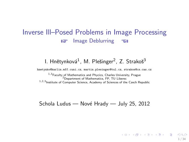
Inverse IllPosed Problems in Image Processing Image Deblurring a - PowerPoint PPT Presentation
Inverse IllPosed Problems in Image Processing Image Deblurring a 1 , M. Ple singer 2 , Z. Strako s 3 I. Hn etynkov hnetynko@karlin.mff.cuni.cz , martin.plesinger@tul.cz , strakos@cs.cas.cz 1 , 3 Faculty of Mathematics and
Inverse Ill–Posed Problems in Image Processing Image Deblurring � � a 1 , M. Pleˇ singer 2 , Z. Strakoˇ s 3 I. Hnˇ etynkov´ hnetynko@karlin.mff.cuni.cz , martin.plesinger@tul.cz , strakos@cs.cas.cz 1 , 3 Faculty of Mathematics and Phycics, Charles University, Prague 2 Department of Mathematics, FP, TU Liberec 1 , 2 , 3 Institute of Computer Science, Academy of Sciences of the Czech Republic Schola Ludus — Nov´ e Hrady — July 25, 2012 1 / 34
Goals of this lecture ◮ What is the inverse ill-posed problem? (Image deblurring as an example of such problem.) ◮ What is the regularization? How / why it works? 2 / 34
Motivation. A gentle start ... What is it an inverse problem? 3 / 34
Motivation. A gentle start ... What is it an inverse problem? Inverse problem A − 1 Forward problem A observation b A ( x ) = b unknown x [Kjøller: M.Sc. thesis, DTU Lyngby, 2007]. 3 / 34
More realistic examples of inverse ill-posed problems Computer tomography in medical sciences Computer tomograph (CT) maps a 3D object of M × N × K voxels by ℓ X-ray measurements on ℓ pictures with m × n pixels, ℓ � : R M × N × K − R m × n . A ( · ) ≡ → j =1 Simpler 2D tomography problem leads to the Radon transform . The inverse problem is ill-posed. (3D case is more complicated.) The mathematical problem is extremely sensitive to errors which are always present in the (measured) data: discretization error (finite ℓ , m , n ); rounding errors ; physical sources of noise (electronic noise in semiconductor PN-junctions in transistors, ...). 4 / 34
More realistic examples of inverse ill-posed problems Transmision computer tomography in crystalographics Reconstruction of an unknown orientation distribution function (ODF) of grains in a given sample of a polycrystalline matherial, ⎛ ⎞ ⎛ ⎞ ⎜ ⎟ ⎜ ⎟ A ⎠ ≡ − → , . . . . ⎜ ⎟ ⎜ ⎟ ⎝ ⎝ ⎠ � �� � observation = data + noise The right-hand side is a set of measured difractograms. [Hansen, Sørensen, S¨ udk¨ osd, Poulsen: SIIMS, 2009]. Further analogous applications also in geology, e.g.: ◮ Seismic tomography (cracks in tectonic plates), ◮ Gravimetry & magnetometry (ore mineralization). 5 / 34
More realistic examples of inverse ill-posed problems General framework In general we deal with a linear problem Ax = b which typically arose as a discretization of a Fredholm integral equation of the 1st kind � � � b ( s ) = K ( s , t ) x ( t ) d t ≡ A x ( t ) , and the right-hand side b is typically contaminated by noise . Our pilot application is the image deblurring problem. 6 / 34
Mathematical model of blurring Image deblurring—Our pilot application Our pilot application is the image deblurring problem [J. Nagy] : ⎛ ⎞ x = true image b = blurred, noisy image ⎜ ⎟ ⎜ ⎟ ⎜ ⎟ ⎜ ⎟ ⎜ ⎟ ⎜ ⎟ A = ⎜ ⎟ ⎜ ⎟ ⎜ ⎟ ⎜ ⎟ ⎜ ⎟ ⎜ ⎟ ⎝ ⎠ It leads to a linear system Ax = b with square nonsingular matrix. We consider gray-scale images, thus each pixel is represetned by one real number, e.g., from the interval [0 , 1] ≡ [black , white]. 7 / 34
Mathematical model of blurring Blurring as an operator of the vector space of images Consider a single-pixel-image (SPI) and a blurring operator A as follows ⎛ ⎞ ⎜ ⎟ A ( X ) = A ⎠ = = B . ⎜ ⎟ ⎝ and denote B = [ b 1 , . . . , b n ] ∈ R m × n . X = [ x 1 , . . . , x n ] , Consider a mapping vec : R m × n − → R mn such that n ] T . x = vec ( X ) ≡ [ x T 1 , . . . , x T The picutre B is called point-spread-function (PSF) . 8 / 34
Mathematical model of blurring Reshaping ⎡ ⎤ B = [ , ,..., b b b ] b = [ ] b B = [ b 1 , . . . , b n ] b 1 1 2 w 1 b . ⎢ . 2 ⎥ b = . ⎣ ⎦ ... b n b w b = vec ( B ) 9 / 34
Mathematical model of blurring Linear and spatial invariant operator Linearity + spatial invariance: + + + + = ↓ ↓ ↓ ↓ ↓ ↓ + + + + = First row: Original (SPI) images (matrices X ). Second row: Blurred (PSF) images (matrices B = A ( X )). 10 / 34
Mathematical model of blurring Matrix A 11 / 34
Mathematical model of blurring Point—spread—function (PSF) Examples of PSF A : horizontal vertical out-of-focus Gaußian motion blur motion blur blur blur (Note: Action of the linear and spatial invariant blurring operator A ( X ) on the given image X is done by 2D convolution of the image with the PSF corresponding to the operator.) 12 / 34
System of linear algebraic equations Smoothing properties If A is linear, then A ( X ) = B , the problem A ( X ) = B can be rewritten as a system of linear algebraic equations A ∈ R mn × mn , x = vec ( X ) , b = vec ( B ) ∈ R mn . Ax = b , The kernel K ( s , t ) in the underlying Fredholm equation � b ( s ) = K ( s , t ) x ( t ) d t , ◮ has smoothing property , ◮ thus the function b ( s ) is smooth (recall the blurred image). Because A and b are restrictions of K ( s , t ), and y ( s ); the linear system Ax = b in some sense inherits these properties. 13 / 34
System of linear algebraic equations Singular valued decomposition For any matrix A ∈ R M × N , r = rank ( A ) there exist orthogonal matrices U − 1 = U T U = [ u 1 , . . . , u M ] ∈ R M × M , V − 1 = V T V = [ v 1 , . . . , v N ] ∈ R N × N , and diagonal matrix Σ = diag ( σ 1 , . . . , σ N ) ∈ R M × N , σ 1 ≥ . . . ≥ σ r > 0 with r positive nonincreasing entries on the diagonal, such that A = U Σ V T , A = u 1 σ 1 v T + . . . + u r σ r v T . 1 r � �� � � �� � A 1 A r It is called the singular value decomposition (SVD) . (See also the principal component analysis (PCA).) 14 / 34
System of linear algebraic equations Singular valued decomposition T A U � V A 1 + A 2 A + ... + A r -1 + A r r � A i A = i = 1 15 / 34
System of linear algebraic equations Singular valued decomposition In our case the matrix A is square nonsingular (i.e. M = N = r ), and, symmetric positive definite (i.e. the SVD is identical to the spectral decomposition of A ). Using the SVD the soution of A ∈ R N × N , Ax = b , N = mn , can be written as u T j b � N x = A − 1 b = V Σ − 1 U T b = v j . σ j j =1 Recall that σ 1 ≥ σ 2 ≥ . . . ≥ σ N > 0. 16 / 34
Properties of the problem The Discrete Picard condition (DPC) The singular values σ j of A decay but the sum u T j b � N x = v j σ j j =1 represents some “real data”. By the (discrete) Picard condition : the projections | u T j b | has to decay on average faster than σ j . σ j , double precision arithmetic 0 10 σ j , high precision arithmetic |(b exact , u j )|, high precision arithmetic −10 10 −20 10 −30 10 −40 10 0 10 20 30 40 50 60 singular value number 17 / 34
Properties of the problem Singular vectors of A Left singular vectors of A represent bases with increasing frequencies: u 1 u 2 u 3 u 4 u 5 u 6 0.1 0.1 0.1 0.1 0.1 0.1 0 0 0 0 0 0 −0.1 −0.1 −0.1 −0.1 −0.1 −0.1 0 200 400 0 200 400 0 200 400 0 200 400 0 200 400 0 200 400 u 7 u 8 u 9 u 10 u 11 u 12 0.1 0.1 0.1 0.1 0.1 0.1 0 0 0 0 0 0 −0.1 −0.1 −0.1 −0.1 −0.1 −0.1 0 200 400 0 200 400 0 200 400 0 200 400 0 200 400 0 200 400 (1D ill-posed problem SHAW(400) [Regularization Toolbox]). 18 / 34
Properties of the problem Right singular vectors ≡ Singular images Reshaped right singular vectors of A (singular images) (Image deblurring problem, Gaußian blur, zero BC). 19 / 34
Impact of noise Noise, Sources of noise Consider a problem of the form b = b exact + b noise , � b exact � ≫ � b noise � , Ax = b , where b noise is unknown and represents, e.g., ◮ rounding errors, ◮ discretization error, ◮ noise with physical sources. We want to compute (approximate) x exact ≡ A − 1 b exact . The vector b noise typically resebles white noise , i.e. it has flat frequency characteristics. 20 / 34
Impact of noise Violation of the discrete Picard condition Recall that the singular vectors of A represent frequencies. Thus the white noise components in left singular subspaces are about the same order of magnitude. The vector b noise violates the discrete Picard condition . Summarizing: ◮ b exact has some real pre-image x exact , it satifies DPC ◮ b noise does not have any real pre-image, it violates DPC. 21 / 34
Impact of noise & regularization Violation of the discrete Picard condition Violation of the discrete Picard condition by noise (SHAW(400)): 5 10 σ j |(b, u j )| for δ noise = 10 −14 0 10 |(b, u j )| for δ noise = 10 −8 |(b, u j )| for δ noise = 10 −4 −5 10 −10 10 −15 10 −20 10 0 50 100 150 200 250 300 350 400 singular value number 22 / 34
Impact of noise & regularization Violation of the discrete Picard condition Consider the naive solution x = A − 1 b = A − 1 b exact + A − 1 b noise , using the singular value expansion u T j b � N x = A − 1 b = v j σ j j =1 u T j b exact u T j b noise � N � N = + v j v j . σ j σ j j =1 j =1 � �� � � �� � x exact amplified noise Thus, even for � b exact � ≫ � b noise � , � A − 1 b exact � ≪ � A − 1 b noise � , the data are covered by the inverted noise. 23 / 34
Regulaization � MatLab demo � 24 / 34
Recommend
More recommend
Explore More Topics
Stay informed with curated content and fresh updates.
