Exiting from QE Fumio Hayashi and Junko Koeda for presentation at - PowerPoint PPT Presentation
Exiting from QE Fumio Hayashi and Junko Koeda for presentation at SF Fed Conference March 28, 2014 Fumio Hayashi and Junko Koeda Exiting from QE March 28, 2014, 1 / 29 To get started...
Exiting from QE Fumio Hayashi and Junko Koeda for presentation at SF Fed Conference March 28, 2014 Fumio Hayashi and Junko Koeda Exiting from QE March 28, 2014, 1 / 29
To get started... ���������������������������������������������� ������ �� � ��������� ���� ����� � � � � � � � � � � � � � � � � � � � � � � � � � � � � � � � � � � � � � � � � � � � � � � � � � � � � � � � � � � � � � � � � � � � � � � � � � � � � � � � � � � � � � � � � � � � � � � � � � � � � � � � � � � � � � � � � � � � � � � � � � � � � � � � � � � � � � � � � � � � � � � � � � � � � � � � � � � � � � � � � � � � � � � � � � � � � � � � � � � � � � � � � � � � � � � � � � � � � � � � � � � � � � � � � � � � � � � � � � � � � � � � � � � � � � � � � � � � � � � � � � � � � � � � � � � � � � � � � � � � � � Fumio Hayashi and Junko Koeda Exiting from QE March 28, 2014, 2 / 29
What This Paper Does Study the effect of QE on macro variables (inflation and GDP) on Japanese data using SVAR (structural VAR) ◮ Japan has, by our count, 130 QE months (as of Dec. 2012) ◮ Includes actual lift-off. Unique in two respects: ◮ Observable and endogenous regimes (unlike in the hidden-state Markov switching model) ◮ IR (impulse response) to regime changes. Fumio Hayashi and Junko Koeda Exiting from QE March 28, 2014, 3 / 29
Plan of Talk Identifying the Regime The Model Estimation Results IR (impulse response) and Counter-factual Analyses Conclusions about BOJ’s Zero-Rate/QE Policy Fumio Hayashi and Junko Koeda Exiting from QE March 28, 2014, 4 / 29
Three QE Spells Z (zero-rate regime) if r (the policy rate) < 0 . 05% (5 basis points). P (normal regime) otherwise. Z = QE because excess reserves > 0 when Z . Periods of Z (Zero-Rate/QE) Regime ◮ QE1: March 1999 - July 2000 ◮ QE2: March 2001 - June 2006 ◮ QE3: December 2008 to date Agrees with BOJ annoucements. For example, ◮ July 14, 2006: “... the BOJ decided ... to change the guideline for money market operations.... The BOJ will encourage the uncollateralized overnight rate to remain at around 0.25 percent.” Fumio Hayashi and Junko Koeda Exiting from QE March 28, 2014, 5 / 29
Policy Rate ( r ) in Japan, 1988 - 2012 9 8 7 6 percent per year 5 4 3 2 1 0 Jan 90 Jan 95 Jan 00 Jan 05 Jan 10 Fumio Hayashi and Junko Koeda Exiting from QE March 28, 2014, 6 / 29
The Exit Condition (to repeat) Periods of Zero-Rate/QE Regime ◮ QE1: March 1999 - July 2000 ◮ QE2: March 2001 - June 2006 ◮ QE3: December 2008 to date During QE’s, BOJ made the inflation commitment. For example ◮ September 21, 1999: “The BOJ ... is explicitly committed to continue this policy [the zero-rate policy] until deflationary concerns subside.” Fumio Hayashi and Junko Koeda Exiting from QE March 28, 2014, 7 / 29
The Model, step 1 of 4: a textbook block-recursive SVAR Point of departure: textbook 3-variable SVAR (see Stock and Watson, J. of Econ. Perspectives , 2001) ◮ ( p , x , r ), p = inflation rate, x = output gap, r = policy rate. ◮ The first two equations are reduced forms in ( p , x ). ◮ The third equation is the Taylor rule, relating r to contemporaneous ( p , x ). 1 Taylor rule: with π t ≡ 12 ( p t + · · · + p t − 11 ), [ ] π t r + β ∗ ′ r t = ρ r r ∗ t + (1 − ρ r ) r t − 1 + σ r v rt , r ∗ t ≡ α ∗ v rt ∼ N (0 , 1) . , r x t (1 × 2) � �� � “desired Taylor rate” ◮ The inflation rate in the Taylor rule is the year-on-year (12-month) inflation rate π . Fumio Hayashi and Junko Koeda Exiting from QE March 28, 2014, 8 / 29
The Model, step 2 of 4: Add the Zero Lower Bound Impose the lower bound: [ ] ρ r r ∗ r t = max t + (1 − ρ r ) r t − 1 + σ r v rt , 0 , v rt ∼ N (0 , 1) . � �� � “shadow Taylor rate” Equivalently, shadow Taylor rate if s t = P , P if shadow Taylor rate > 0 , r t = s t = otherwise. 0 if s t = Z . Z Note: ◮ The regime s t is endogenous. ◮ s t = Z if and only if r t = 0 (the econometrician doesn’t have to observe the shadow Taylor rate). Fumio Hayashi and Junko Koeda Exiting from QE March 28, 2014, 9 / 29
The Model, step 3 of 4: Introduce Exit Condition If s t − 1 = Z , P if shadow Taylor rate > 0 and π t > π + σ π v π t , � �� � s t = target inflation rate otherwise. Z If s t − 1 = P , as before, i.e., P if shadow Taylor rate > 0 , s t = otherwise. Z 1 (reminder) π t ≡ 12 ( p t + · · · + p t − 11 ), [ ] π t ′ r + β ∗ shadow Taylor rate = ρ r r ∗ t + (1 − ρ r ) r t − 1 + σ r v rt , r ∗ t ≡ α ∗ . r x t (1 × 2) � �� � “desired Taylor rate” Fumio Hayashi and Junko Koeda Exiting from QE March 28, 2014, 10 / 29
The Model, step 4 of 4: Add m Add m to ( p , x , r ). 0 if s t = P , m t = [ ] v mt ∼ N (0 , 1) max m st , 0 , if s t = Z , where [ ] π t ′ m st ≡ α s + β s + γ s m t − 1 + σ s v st , x t (reminder) ◮ p ≡ monthly inflation rate, π t ≡ 1 12 ( p t + · · · + p t − 11 ), ◮ x ≡ output gap, ( ) actual reserves ◮ m ≡ log . required reserves Fumio Hayashi and Junko Koeda Exiting from QE March 28, 2014, 11 / 29
Plan of Talk Identifying the Regime The Model Estimation Results IR (impulse response) and Counter-factual Analyses Conclusions about BOJ’s Zero-Rate/QE Policy Fumio Hayashi and Junko Koeda Exiting from QE March 28, 2014, 12 / 29
Estimation: The Monthly Data p (monthly CPI inflation rate) π (12-month inflation rate) ( ) actual reserves t m (excess reserve rate): m t ≡ 100 × log . required reserves t r (policy rate): collateralized overnight interbank rate. x (GDP gap): monthly interpolation of official quarterly estimate. Fumio Hayashi and Junko Koeda Exiting from QE March 28, 2014, 13 / 29
12-Month Inflation Rate ( π ), 1988-2012 4 3 2 percent per year 1 0 −1 −2 Jan 90 Jan 95 Jan 00 Jan 05 Jan 10 Fumio Hayashi and Junko Koeda Exiting from QE March 28, 2014, 14 / 29
GDP, 1988-2012 log actual GDP potential log GDP Jan 90 Jan 95 Jan 00 Jan 05 Jan 10 Fumio Hayashi and Junko Koeda Exiting from QE March 28, 2014, 15 / 29
Estimation: The Equations bivariate ( p , x ) reduced form: allowed to shift between (lagged) P (normal regime) and (lagged) Z (zero-rate/QE regime) by Lucas. Taylor rule: estimated on P + Z , regime endogeneity taken into account. Excess reserve supply equation: on Z = { QE1, QE2, QE3 } , but QE1 dropped because QE1 looks different. Fumio Hayashi and Junko Koeda Exiting from QE March 28, 2014, 16 / 29
Estimation: ( p , x ) Reduced Form ( t value in brackets) sample period is January 1992 - December 2012 subsample P ( s t − 1 = P , sample size = 123) R 2 dep. var. const. p t − 1 x t − 1 r t − 1 m t − 1 − 0 . 23 0 . 10 0 . 14 0 . 39 0.19 p t [1 . 1] [1 . 7] [3 . 4] [ − 0 . 9] − 0 . 20 − 0 . 00 x t 0 . 93 0 . 02 0.80 [ − 1 . 4] [ − 0 . 1] [21] [0 . 3] subsample Z ( s t − 1 = QE2+QE3 , sample size = 112) R 2 dep. var. const. p t − 1 x t − 1 r t − 1 m t − 1 0 . 15 0 . 22 0 . 16 0 . 0002 0.11 p t [0 . 3] [2 . 4] [1 . 8] [0 . 1] − 1 . 21 − 0 . 02 0 . 77 0 . 0052 0.75 x t [14] [2 . 6] [ − 3 . 3] [ − 0 . 3] Fumio Hayashi and Junko Koeda Exiting from QE March 28, 2014, 17 / 29
Things to Note about Estimated Reduced Form subsample s t − 1 = P : ◮ lagged r coefficient in p t equation positive and significant. subsample s t − 1 = Z (QE2+QE3): ◮ lagged m coefficient in p t and x t equations positive. ◮ Intercepts lower for Z than for P . Fumio Hayashi and Junko Koeda Exiting from QE March 28, 2014, 18 / 29
Plan of Talk Identifying the Regime The Model Estimation Results IR (impulse response) and Counter-factual Analyses Conclusions about BOJ’s Zero-Rate/QE Policy Fumio Hayashi and Junko Koeda Exiting from QE March 28, 2014, 19 / 29
Recommend
More recommend
Explore More Topics
Stay informed with curated content and fresh updates.
