EUCLIDEAN SPACES and CONVERGENCE IN R n Summary of lecture notes - PowerPoint PPT Presentation
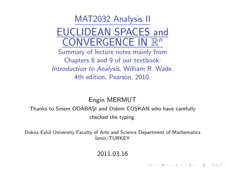
MAT2032 Analysis II EUCLIDEAN SPACES and CONVERGENCE IN R n Summary of lecture notes mainly from Chapters 8 and 9 of our textbook: Introduction to Analysis , William R. Wade. 4th edition, Pearson, 2010. Engin MERMUT Thanks to Sinem ODABAS I
Other important norms on R n that give the same topology For each x = ( x 1 , x 2 , . . . , x n ) in the n -dimensional Euclidean space R n , ◮ The ℓ 1 -norm (read L-one-norm) of x = ( x 1 , x 2 , . . . , x n ) is the scalar n � � x � 1 = | x 1 | + | x 2 | + · · · + | x n | = | x k | . k =1 ◮ The sup-norm of x = ( x 1 , x 2 , . . . , x n ) is the scalar � x � ∞ = max( {| x 1 | , | x 2 | , . . . , | x n |} ) . The relationship between the Euclidean norm, ℓ 1 -norm and sup-norm is given by the following inequalities: Proposition For every x = ( x 1 , x 2 , . . . , x n ) in R n , we have ◮ | x k | ≤ � x � ∞ ≤ � x � ≤ √ n � x � ∞ for each k = 1 , 2 , . . . , n , and ◮ � x � ≤ � x � 1 ≤ n � x � ∞ ≤ n � x � .
These inequalities are easily obtained since for each k = 1 , 2 , . . . , n , | x k | 2 ≤ � x � 2 = x 2 1 + x 2 2 + · · · + x 2 n ≤ n (max( {| x 1 | , | x 2 | , . . . , | x n |} )) = n � x � 2 ∞ , and � x � 2 = | x 1 | 2 + | x 2 | 2 + · · · + | x n | 2 ≤ ( | x 1 | + | x 2 | + · · · + | x n | ) 2 = � x � 2 1 . The important thing for all these three norms is that because of these inequalities, the “ metrics ” that they induce on R n give the same collection of “ open sets ”, so although they are different metrics, they give R n the same topology . These inequalities will also be useful when we need some inequalities between the coordinates of the vector x and the norm of the vector x .
Lines, line segments and parallelograms in R n Let a and b be vectors in R n . We define: ◮ The (straight) line in R n that passes through the point a in the direction of the vector b � = 0 is the set of points ℓ a ( b ) = { a + t b | t ∈ R } . ◮ The line segment from the point a to the point b � = a in R n is the set of points L ( a ; b ) = { (1 − t ) a + t b | t ∈ [0 , 1] } . ◮ The entire parallelogram (with its boundary and the region it surrounds) spanned by the vectors a and b is the set of points P ( a , b ) = { u a + t b | u , v ∈ [0 , 1] } .
Hyperplanes in R n Lines in R 2 and planes in R 3 are generalized to hyperplanes in R n : It will be “flat” in some sense and will have dimension n − 1. A hyperplane passing through a point a ∈ R n with a normal b � = 0 is defined to be the set Π b ( a ) = { x ∈ R n | ( x − a ) · b = 0 } , that is, it consists of all points x ∈ R n such that x − a is orthogonal to b . If b = ( b 1 , b 2 , . . . , b n ) and d = a · b , then the hyperplane Π b ( a ) consists of all x = ( x 1 , x 2 , . . . , x n ) ∈ R n such that b 1 x 1 + b 2 x 2 + . . . b n x n = d . This gives a linear equation for the hyperplane.
Linear transformations A function T : R n → R m is said to be linear if for all x , y ∈ R n and for all scalars α ∈ R , T ( x + y ) = T ( x ) + T ( y ) and T ( α x ) = α T ( x ) . Linear functions T : R n → R m are also called linear transformations or linear operators . The set of all linear transformations from R n to R m is denoted by L ( R n ; R m ) . You are studying linear transformations in your Linear Algebra course. You all know well operations on matrices. See also Appendix C Matrices and Determinants (pages 629–636) of your textbook. We shall use elementary linear algebra as summarized below.
Review elementary linear algebra Note that your textbook uses the notation B = [ b ij ] m × n to denote an m × n matrix whose ( i , j )th entry, that is, the entry in the intersection of i th row and j th column is b ij instead of our longer notation B = [ b ij ] m , n i , j =1 . Anyway, what is meant is just the m × n matrix b 11 b 12 · · · b 1 n b 21 b 22 · · · b 2 n B = [ b ij ] m × n = [ b ij ] m , n i , j =1 = . . . . ... . . . . . . b m 1 b m 2 · · · b mn For the elementary linear algebra part that we shall use be sure that you know the following: ◮ The algebra of matrices (product, sum, the m × n zero matrix 0 = 0 m × n , the n × n identity matrix I = I n × n , etc.). ◮ Inverse of a matrix. ◮ Properties of determinants, the expansion of a determinant along a row or a column by minors. ◮ det( AB ) = det( A ) det( B ) for all n × n matrices A and B .
◮ An n × n matrix is invertible if and only if det( A ) � = 0. ◮ The transpose of a matrix B is denoted by B T . ◮ The adjoint of an n × n matrix B is the transpose of the matrix of cofactors of B , that is, [( − 1) i + j det( B ij )] n adj( B ) is the transpose of the matrix i , j =1 , where B ij is the matrix obtained from B by deleting the i th row and j th column. ◮ If B is an invertible n × n matrix, then 1 B − 1 = det( B ) adj( B ) . ◮ Cramer’s rule for the solution of a linear system of equations whose coefficients matrix has nonzero determinant. ◮ For each linear transformation T : R n → R m , when you fix a basis for R n and a bases for R m , then there is a matrix representing this linear transformation in these basis for R n and R m .
The matrix representing a linear transformation Theorem There is a one-to-one correspondence between the set L ( R n ; R m ) of all linear transformations from R n to R m and the set of all m × n matrices via the following: For each linear transformation T : R n → R m , there exists a unique m × n matrix B such that for each x = ( x 1 , x 2 , . . . , x n ) ∈ R n , we have T ( x ) = y where y = ( y 1 , y 2 , . . . , y m ) ∈ R m is such that x 1 y 1 x 2 y 2 B = . . . . . . . x n y m Here the m × n matrix B = [ b ij ] m , n i , j =1 is such that for each j = 1 , 2 , . . . , n, the jth column of B is the coordinates of T ( e j ) , where { e 1 , e 2 , . . . , e n } is the usual standard basis for R n : T ( e j ) = ( b 1 j , b 2 j , . . . , b mj ) , j = 1 , 2 , . . . , n .
All linear transformations are of the form T ( x ) = B x By abusing notation for our usage, we shall identify points x = ( x 1 , x 2 , . . . , x n ) with 1 × n row matrices or n × 1 column matrices by setting � � [ x ] = x 1 x 2 · · · x n or its transpose x 1 x 2 � T = � [ x ] = x 1 x 2 · · · x n . . . . x n Moreover, we shall write B x for the product of the m × n matrix B and the n × 1 column matrix [ x ]. So with this agreement in the abuse of notation T ( x ) = B x .
If T : R n → R m and U : R m → R p are linear transformations, then so is their composition U ◦ T : R n → R p . Moreover, if B is the m × n matrix that represents T and C is the p × m matrix that represents U , then the matrix product CB is the matrix that represents U ◦ T . Indeed, this is the reason why multiplication of matrices have been defined in the way you all know well. Note that with our above agreement on notation, we have: for all x ∈ R n , T ( x ) = B x for all y ∈ R m . U ( y ) = C y Thus we obtain that for all x ∈ R n , ( U ◦ T )( x ) = U ( T ( x )) = C [ T ( x )] = CB x .
Note also that our identification of the points x = ( x 1 , x 2 , . . . , x n ) with 1 × n row matrices or n × 1 column matrices by setting � � [ x ] = x 1 x 2 · · · x n or its transpose x 1 x 2 � T = � [ x ] = x 1 x 2 · · · x n . . . x n have the following properties: For all vectors x , y ∈ R n and scalars α ∈ R , ◮ [ x + y ] = [ x ] + [ y ], ◮ [ x · y ] = [ x ][ y ] T , ◮ [ α x ] = α [ x ].
Linear transformations are needed to study differentiable functions f : R n − → R m We shall use the above summarized notation for linear transformations when we study differentiable functions from R n to R m . The idea is the same as in the one variable case: The derivative of a function f : R → R at a point a ∈ R gives the tangent line at this point and we locally approach f by the linear function g : R → R defined by g ( x ) = f ′ ( a )( x − a ) + f ( a ), x ∈ R . The multidimensional analogue of this will replace f ′ ( a ) (and so the linear function g ) by a linear transformation T : R n → R m (or the matrix representing this linear transformation). The “derivative” of the function f : R n → R m at a point a = ( a 1 , a 2 , . . . , a n ) ∈ R n will be the “Jacobian matrix” of the function f : R n → R m , that is, the matrix of partial derivatives, evaluated at the point a = ( a 1 , a 2 , . . . , a n ). This matrix will be called the total derivative of f at the point a .
More precisely, if for all x = ( x 1 , x 2 , . . . , x n ) ∈ R n , f ( x ) = ( f 1 ( x ) , f 2 ( x ) , . . . , f m ( x )) ∈ R m , then the derivative of the function f : R n → R m at the point a = ( a 1 , a 2 , . . . , a n ) will be the linear transformation T : R n → R m that is represented by the matrix of partial derivatives evaluated at the point a = ( a 1 , a 2 , . . . , a n ), that is, the m × n matrix ∂ f 1 ∂ f 1 ∂ f 1 · · · ∂ x 1 ∂ x 2 ∂ x n � ∂ f i � m , n ∂ f 2 ∂ f 2 ∂ f 2 · · · = . ∂ x 1 ∂ x 2 ∂ x n ∂ x j i , j =1 . . . ... . . . . . . ∂ f m ∂ f m ∂ f m · · · ∂ x 1 ∂ x 2 ∂ x n of partial derivatives evaluated at the point a = ( a 1 , a 2 , . . . , a n ). When studying differentiability, we shall also use the operator norm of a linear transformation:
The operator norm of a linear transformation T : R n → R m Theorem Let T ∈ L ( R n ; R m ) , that is, T : R n → R m is a linear transformation. 1. There exists a real number C > 0 such that � T ( x ) � ≤ C � x � for all x ∈ R n . 2. The set { C ∈ R | C > 0 and for all x ∈ R n , � T ( x ) � ≤ C � x �} of positive real numbers is nonempty by the first part and so it has a greatest lower bound which is called the operator norm of T, denoted by � T � : � T � = inf( { C ∈ R | C > 0 and for all x ∈ R n , � T ( x ) � ≤ C � x �} ) . It satisfies � T ( x ) � ≤ � T �� x � for all x ∈ R n . Let B be the m × n matrix that represents T so that T ( x ) = B x for all x ∈ R n . Then the operator norm � B � of the matrix B is also defined to be � T � .
Proof. Let B be the m × n matrix that represents T so that T ( x ) = B x for all x ∈ R n . The result is clear if B = 0. So assume that B � = 0. Let b 1 , b 2 , . . . , b m be the rows of the matrix B . We then have that for all x ∈ R n , T ( x ) = B x = ( b 1 · x , b 2 · x , . . . , b m · x ) . Now by Cauchy-Schwarz inequality, we obtain that ( b 1 · x ) 2 + ( b 2 · x ) 2 + · · · + ( b m · x ) 2 � T ( x ) � 2 = ( � b 1 �� x � ) 2 + ( � b 2 �� x � ) 2 + · · · + ( � b m �� x � ) 2 ≤ m · [max( {� b 1 � 2 , � b 2 � 2 , . . . , � b m � 2 } )] � x � 2 = K � x � 2 , ≤ where K = m · [max( {� b 1 � 2 , � b 2 � 2 , . . . , � b m � 2 } )] is a finite √ positive real number since B � = 0. So for C = K > 0, we have that � T ( x ) � ≤ C � x � for all x ∈ R n . Thus � T � is a finite nonnegative real number. By definition of � T � as the infimum of the set { C ∈ R | C > 0 and for all x ∈ R n , � T ( x ) � ≤ C � x �} , there exists a sequence ( C k ) ∞ k =1 of positive real numbers in this set such that lim k →∞ C k = � T � . Thus we have that for all k ∈ Z + and all x ∈ R n , � T ( x ) � ≤ C k � x � . Taking limit as k → ∞ , we obtain that � T ( x ) � ≤ � T �� x � for all x ∈ R n .
Open and closed sets in R n Open and closed balls and spheres are defined as follows: ◮ For a point a in R n and a real number r > 0, B r ( a ) = ( open ball with center at a and radius r ) { x ∈ R n |� x − a � < r } . = ◮ For a point a in R n and a real number r ≥ 0, B r ( a ) = ( closed ball with center at a and radius r ) { x ∈ R n |� x − a � ≤ r } . = ◮ For a point a in R n +1 and a real number r > 0, S n r ( a ) = ( n -dimensional sphere with center at a and radius r ) { x ∈ R n +1 |� x − a � = r } . = A subset U ⊆ R n is said to be open if for each point a in the subset U , there exists a real number r > 0 such that B r ( a ) ⊆ U , that is, each point a ∈ U is surrounded by an open ball lying wholly in U . A subset K ⊆ R n is said to be closed if its complement R n \ K is an open set in R n .
Examples of open and closed sets 1. For a point a in R n and a real number r > 0, the open ball B r ( a ) is open. 2. For a point a in R n and a real number r ≥ 0, the closed ball B r ( a ) is closed. 3. For a point a in R n +1 and a real number r > 0, the n -dimensional sphere S n r ( a ) is closed. 4. For each point a ∈ R n , the singleton { a } is closed and R n \ { a } is open. 5. The empty set ∅ and the whole space R n are both open and closed. Question: A set in R n that is both open and closed is said to be a clopen set. Are there any clopen subsets of R n except ∅ and R n ? This is indeed the question whether R n is connected or not. See the part on connected subsets of R n .
Union and intersection of open sets Theorem ◮ Union of any collection of open sets (maybe an infinite collection of open sets) in R n is open. ◮ Intersection of finitely many open sets in R n is open. That is: ◮ If { V α } α ∈ A is an indexed collection of open subsets of R n , then � V α is open . α ∈ A ◮ If p ∈ Z + and V 1 , V 2 , . . . , V p are finitely many open subsets of R n , then p � V k = V 1 ∩ V 2 ∩ · · · ∩ V p is open . k =1
Union and intersection of closed sets Theorem ◮ Intersection of any collection of closed sets (maybe an infinite collection of closed sets) in R n is closed. ◮ Union of finitely many closed sets in R n is closed. That is: ◮ If { E α } α ∈ A is an indexed collection of closed subsets of R n , then � E α is closed . α ∈ A ◮ If p ∈ Z + and E 1 , E 2 , . . . , E p are finitely many closed subsets of R n , then p � E k = E 1 ∪ E 2 ∪ · · · ∪ E p is closed . k =1
Interior, exterior and boundary points For a set E ⊆ R n and a point a ∈ R n , a is said to be ◮ an interior point of E if there exists a real number r > 0 such that B r ( a ) ⊆ E , ◮ an exterior point of E if there exists a real number r > 0 such that B r ( a ) ⊆ R n \ E , ◮ a boundary point of E if for every real number r > 0, B r ( a ) ∩ ( R n \ E ) � = ∅ . B r ( a ) ∩ E � = ∅ and So a set E ⊆ R n divides the whole space R n into three disjoint pieces, two of which is open and the boundary is closed: � � R n = int( E ) ∂ E ext( E ) ���� � �� � � �� � all boundary points = E o =all interior points all exterior points � �� � = E =closure of E To prove this decomposition, we shall of course firstly define the interior and closure of a subset E of R n .
The interior and closure of a subset E of R n Let E ⊆ R n . ◮ The interior of E is the set � E o = int( E ) = { V | V ⊆ E and V is open in R n } . ◮ The closure of E is the set � { C | C ⊇ E and C is closed in R n } . E = Theorem For every E ⊆ R n , we have: 1. E o ⊆ E ⊆ E, E o is open and E is closed. 2. If V is open and V ⊆ E, then V ⊆ E o . So E o is the largest open set contained in E. 3. If C is closed and C ⊇ E, then C ⊇ E. So E is the smallest closed set containing E. 4. E is open if and only if E o = E. 5. E is closed if and only if E = E.
The interior, boundary and closure of a set Now we can prove the result for a subset E ⊆ R n that we stated at the beginning: � � R n = int( E ) ∂ E ext( E ) ���� � �� � � �� � all boundary points = E o =all interior points all exterior points � �� � = E =closure of E To prove the following theorem, firstly show that for every x ∈ R n : ◮ x ∈ E ⇐ ⇒ B r ( x ) ∩ E � = ∅ for all r > 0 . ◮ x �∈ E o ⇐ B r ( x ) ∩ ( R n \ E ) � = ∅ for all r > 0 . ⇒ Theorem Let E ⊆ R n . Then 1. E o is the set of all interior points of E and ext( E ) is the set of all interior points of R n \ E. So ext ( E ) = ( R n \ E ) o . 2. ∂ E = E \ E o and E = E o ∪ ∂ E. 3. ∂ E = E ∩ ( R n \ E ) and ∂ E is closed.
Cluster points (= accumulation points = limit points) of a subset E ⊆ R n Let E ⊆ R n . A point x ∈ R n is said to be a cluster point (or an accumulation point or a limit point ) of the set E if for every real number r > 0, the intersection B r ( x ) ∩ E contains a point other than the point x , that is, ( B r ( x ) \ { x } ) ∩ E � = ∅ for all real numbers r > 0 , equivalently, B r ( x ) ∩ E contains infinitely many points for all real numbers r > 0. Theorem The closure of a subset E ⊆ R n is the union of E and all of its cluster points: E = E ∪ { all cluster points of E } . This holds because for a point x ∈ R n , x ∈ E ⇐ ⇒ B r ( x ) ∩ E � = ∅ for all r > 0 , and so, x ∈ E \ E ⇐ ⇒ ( B r ( x ) \ { x } ) ∩ E � = ∅ for all r > 0 .
Isolated points of a subset E ⊆ R n Let E ⊆ R n . Take a point a in the set E . There are two cases for the point a ∈ E : ◮ The point a ∈ E is a cluster point of E , that is, ( B r ( a ) \ { a } ) ∩ E � = ∅ for all real numbers r > 0 . ◮ The point a ∈ E satisfies ( B δ ( a ) \ { a } ) ∩ E = ∅ for some real number δ > 0 . That is, there exists an open ball with center at the point a ∈ E that contains no other point of E except of course the point a that we have taken from E : B δ ( a ) ∩ E = { a } for some real number δ > 0 . Such a point a ∈ E is said to be an isolated point of E ; it is isolated from all other points of E since an open ball of positive radius with center at a ∈ E contains no other points of E .
Interior, closure and boundary of unions and intersections Theorem Let A and B be subsets of R n . 1. ( A ∪ B ) o ⊇ A o ∪ B o , 2. ( A ∩ B ) o = A o ∩ B o , 3. A ∪ B = A ∪ B, 4. A ∩ B ⊆ A ∩ B, 5. ∂ ( A ∪ B ) ⊆ ∂ A ∪ ∂ B, 6. ∂ ( A ∩ B ) ⊆ ( A ∩ ∂ B ) ∪ ( B ∩ ∂ A ) ∪ ( ∂ A ∩ ∂ B ) ⊆ ∂ A ∪ ∂ B. In the above theorem, for the parts where equality need not hold, give examples where equality does not hold.
Distance of a point to a closed set Theorem Let E be a nonempy subset of R n . Let a ∈ R n . Let d be the distance of the point a to the set E defined by d = inf x ∈ E � x − a � = inf ( {� x − a � | x ∈ E } ) . ◮ If a ∈ E, then clearly d = 0 . ◮ If a �∈ E and E is closed , then d > 0 . So if E is closed , then we have that a ∈ E if and only if d = 0 : Thus the points not in a closed set E are at a positive distance apart form the closed set E . This is because if E is closed and a �∈ E , then R n \ E is open and a ∈ R n \ E which implies the existence of a positive real number r > 0 such that B r ( a ) ⊆ R n \ E , and so B r ( a ) ∩ E = ∅ . Thus for every x ∈ E , we have that x �∈ B r ( a ). So for every x ∈ E , we have � x − a � ≥ r . This implies that d ≥ r . Since r > 0, we obtain d > 0.
Neighborhood of a point a in R n Let a ∈ R n . A subset A ⊆ R n is said to be a neighborhood of a in R n if there exists an open set U in R n such that a ∈ U ⊆ A , equivalently there exists a real number r > 0 such that B r ( a ) ⊆ A . Note that a neighborhood of a point a ∈ R n is not necessarily an open set; but it contains an open set that contains the point a . In some textbooks, a neighborhood is assumed to be open or assumed to be an open ball. What is essential in all these definitions is that a neighborhood of a point a contains an open set that contains a . A deleted neighborhood of a point a ∈ R n is a neighborhood of a minus the point a itself, that is, A \ { a } for a neighborhood A of a . Open sets and neighborhoods are used to state limits and continuity.
Limit of a sequence in terms of open sets Let { x k } ∞ k =1 be a sequence of points in R n . Let a ∈ R n . The sequence { x k } ∞ k =1 is said to converge to the point a if for every real number ǫ > 0, there exists a positive integer N such that for all integers k , k ≥ N = ⇒ � x k − a � < ǫ. Notice that this last condition means that x k ∈ B ǫ ( a ). So we have: Theorem k =1 in R n and a point a ∈ R n , the following For a sequence { x k } ∞ are equivalent: 1. The sequence { x k } ∞ k =1 converges to the point a . 2. For every open set V that contains a , there exists a positive integer N such that for all integers k ≥ N, x k ∈ V . 3. For every neighborhood A of the point a , there exists a positive integer N such that for all integers k ≥ N, x k ∈ A.
Inverse image of a function Remember that for a function f : A → B from a set A to a set B , we define for C ⊆ A and D ⊆ B : ◮ The image of C under f is the set f ( C ) = { f ( x ) | x ∈ C } that consists of the images of every element in the set C . ◮ The inverse image of the set D is the set f − 1 ( D ) = { x ∈ A | f ( x ) ∈ D } that consists of all elements from A whose image is in the set D . Never mix this notation with the inverse of a function. The above inverse image f − 1 ( D ) is defined for every function f : A → B and D ⊆ B . But as you know well to speak about the inverse function f − 1 : B → A is only possible if the function f : A → B is one-to-one and onto.
Limit of a function in terms of open sets Let a ∈ R n and let V be an open set that contains a . Let f : V \ { a } → R m be a function. Let L ∈ R m . Then f ( x ) is said to converge to L as x approaches a and we write lim x → a f ( x ) = L if for every real number ǫ > 0, there exists a real number δ > 0 such that for all x ∈ R n , 0 < � x − a � < δ = ⇒ � f ( x ) − L � < ǫ. Notice that ◮ 0 < � x − a � < δ means that x ∈ B δ ( a ) \ { a } , ◮ � f ( x ) − L � < ǫ means that f ( x ) ∈ B ǫ ( L ), and so ◮ ∀ x ∈ R n (0 < � x − a � < δ = ⇒ � f ( x ) − L � < ǫ ) means that f ( B δ ( a ) \ { a } ) ⊆ B ǫ ( L ) or B δ ( a ) \ { a } ⊆ f − 1 ( B ǫ ( L )) .
Since lim x → a f ( x ) = L means that ∀ x ∈ R n (0 < � x − a � < δ = ∀ ǫ > 0 ∃ δ > 0 ⇒ � f ( x ) − L � < ǫ ) , which is equivalent to B δ ( a ) \ { a } ⊆ f − 1 ( B ǫ ( L )) , ∀ ǫ > 0 ∃ δ > 0 we obtain: Theorem For a ∈ R n , an open set V that contains a , L ∈ R m and a function f : V \ { a } → R m , the following are equivalent: 1. lim x → a f ( x ) = L. 2. For every open set U in R m that contains L , there exists an open set G that contains a such that G \ { a } ⊆ f − 1 ( U ) . 3. For every neighborhood H of L in R m , there exists a neighborhood A of a in R n such that A \ { a } ⊆ f − 1 ( H ) . 4. For every neighborhood H of L in R m , there exists a deleted neighborhood K of a in R n such that K ⊆ f − 1 ( H ) .
Continuity of a function at a point in terms of open sets Let E ⊆ R n and let f : E → R m be a function. Let a ∈ E . The function f is said to be continuous at the point a if for every real number ǫ > 0, there exists a real number δ > 0 such that for all x ∈ R n , � x − a � < δ and x ∈ E ⇒ � f ( x ) − f ( a ) � < ǫ. = Notice that ◮ � x − a � < δ means that x ∈ B δ ( a ), ◮ � f ( x ) − f ( a ) � < ǫ means that f ( x ) ∈ B ǫ ( f ( a )), and so ◮ ∀ x ∈ E ( � x − a � < δ = ⇒ � f ( x ) − f ( a ) � < ǫ ) means that f ( E ∩ B δ ( a )) ⊆ B ǫ ( f ( a )) or E ∩ B δ ( a ) ⊆ f − 1 ( B ǫ ( f ( a ))) . We say that the function f : E → R m is a continuous function if f is continuous at every point a ∈ E .
Since f : E → R m is continuous at a point a ∈ E ⊆ R n means that ∀ ǫ > 0 ∃ δ > 0 ∀ x ∈ E ( � x − a � < δ = ⇒ � f ( x ) − f ( a ) � < ǫ ) , which is equivalent to E ∩ B δ ( a ) ⊆ f − 1 ( B ǫ ( f ( a ))) , ∀ ǫ > 0 ∃ δ > 0 we obtain: Theorem For a function f : E → R m and a point a ∈ E ⊆ R n , the following are equivalent: 1. f is continuous at the point a . 2. For every open set U in R m that contains f ( a ) , there exists an open set G that contains a such that E ∩ G ⊆ f − 1 ( U ) . 3. For every neighborhood H of f ( a ) in R m , there exists a neighborhood A of a in R n such that E ∩ A ⊆ f − 1 ( H ) .
Characterization of continuous functions in terms of open sets (and closed sets) Theorem For a function f : R n → R m , the following are equivalent: 1. f : R n → R m is a continuous function, that is, f is continuous at every point a ∈ R n . 2. f − 1 ( V ) is an open subset of R n for every open subset V of R m . 3. f − 1 ( K ) is a closed subset of R n for every closed subset K of R m . By this theorem, continuity of a function is stated easily in terms of inverse images of open sets. What does happen for a function f : E → R m when E ⊆ R n but E � = R n ? How can we state the similar result? The answer will be to use relatively open and relatively closed subsets of E defined as follows:
Relatively open and relatively closed sets in E ⊆ R n Let E ⊆ R n . ◮ A subset U ⊆ E is said to be relatively open in E if U = V ∩ E for some open set V in R n . ◮ A subset K ⊆ E is said to be relatively closed in E if K = C ∩ E for some closed set C in R n . Theorem For a function f : E → R m where E ⊆ R n , the following are equivalent: 1. f : E → R m is a continuous function, that is, f is continuous at every point a ∈ E. 2. f − 1 ( V ) is a relatively open subset of E for every open subset V of R m . 3. f − 1 ( K ) is a relatively closed subset of E for every closed subset K of R m .
Theorem Let E ⊆ R n and let U ⊆ E . 1. U is relatively open in E if and only if for each a ∈ U, there exists a real number r > 0 such that B r ( a ) ∩ E ⊆ U. 2. If E is an open subset of R n , then U is relatively open in E if and only if U is open in R n . 3. If E is a closed subset of R n , then U is relatively closed in E if and only if U is closed in R n .
Characterization of continuity of a function f : E → F in terms of relatively open and relatively closed sets Theorem For a function f : E → F where E ⊆ R n and F ⊆ R m , the following are equivalent: 1. f : E → F is a continuous function, that is, f is continuous at every point a ∈ E. 2. f − 1 ( V ) is a relatively open subset of E for every relatively open subset V of F. 3. f − 1 ( K ) is a relatively closed subset of E for every relatively closed subset K of F.
Restriction of continuous functions are continuous Theorem Let f : E → R m be a function where E ⊆ R n . Let H ⊆ E and let Y ⊆ R m be such that f ( H ) ⊆ Y . Let g : H → Y be the restriction of the function f obtained by restricting the domain of f to H and the range of f to Y : g : H → Y defined by g ( x ) = f ( x ) for all x ∈ H . We can define g in this way since f ( H ) ⊆ Y . If f : E → R m is a continuous function, then its restriction g : H → Y is also a continuous function.
Closure of a set E ⊆ R n in terms of convergent sequences in E Theorem Let E ⊆ R n . 1. The closure of E consists of limits of all convergent sequences in E: � � k →∞ x k | { x k } ∞ E = lim k =1 is a convergent sequence in E . 2. E is closed if and only E contains all the limits of convergent sequences in E, that is, for every convergent sequence { x k } ∞ k =1 in E, the limit lim k →∞ x k is also in E.
Sequences in R n Let { x k } ∞ k =1 be a sequence of points in R n . ◮ Let a ∈ R n . The sequence { x k } ∞ k =1 is said to converge to the point a if for every real number ǫ > 0, there exists a positive integer N such that for all integers k , k ≥ N = ⇒ � x k − a � < ǫ. In this case, we write x k → a as k → ∞ , or, lim k →∞ x k = a and say that a is the limit of the sequence { x k } ∞ k =1 . ◮ { x k } ∞ k =1 is said to be a convergent sequence if there exists a ∈ R n such that the sequence { x k } ∞ k =1 converges to a . ◮ { x k } ∞ k =1 is said to be a Cauchy sequence if for every real number ǫ > 0, there exists N ∈ Z + such that for all integers k and r , k ≥ N and r ≥ N ⇒ � x k − x r � < ǫ. = ◮ { x k } ∞ k =1 is said to be a bounded sequence if there exists a real number M > 0 such that � x k � ≤ M for all k ∈ Z + .
Limits are taken in each coordinate separately To denote the coordinates of the elements of the sequence { x k } ∞ k =1 in R n , let us write for each k ∈ Z + , x k = ( x k (1) , x k (2) , . . . , x k ( n )) ∈ R n . With this notation: Theorem k =1 be a sequence in R n and let a ∈ R n whose coordinates Let { x k } ∞ are given by a = ( a (1) , a (2) , . . . , a ( n )) ∈ R n and for all k ∈ Z + , x k = ( x k (1) , x k (2) , . . . , x k ( n )) ∈ R n . Then the sequence { x k } ∞ k =1 converges to the point a if and only if for each j = 1 , 2 , . . . , n, the component sequence { x k ( j ) } of real numbers converges to the real number a ( j ) , that is, the sequence of jth coordinates of the sequence { x k } ∞ k =1 converges to the jth coordinate of a for each j = 1 , 2 , . . . , n: k →∞ x k = a lim ⇐ ⇒ k →∞ x k ( j ) = a ( j ) for each j = 1 , 2 , . . . , n . lim
The countable set Q n is dense in R n The subset Q of all rational numbers is dense in R , that is, between any two real numbers, there exists a rational number. Using this, for any real number a , we can find a sequence of rational numbers that converges to a . Doing this componentwise for a point a ∈ R n , we obtain: Theorem k =1 in Q n such that For each a ∈ R n , there is a sequence { x k } ∞ k →∞ x k = a . lim This means that each point of R n is in the closure of the set Q n . Such sets are said to be dense in R n . A subset A of R n is said to be dense in R n if A = R n . Since the set Q n of all points whose coordinates are rational numbers is also a countable set, we have found a countable dense subset of R n which is important for the structure of R n as we shall see in the proof of Lindel¨ of theorem.
Properties of limits of sequences in R n The following results are proved like in the case of sequences of real numbers mainly by just replacing the absolute value | x − a | for real numbers x and a with � x − a � for points x , a ∈ R n . ◮ A sequence in R n can have at most one limit, that is, if a sequence { x k } ∞ k =1 converges to a point a and to a point b , then we must have a = b . So we can speak of the limit of a convergent sequence in R n . k =1 in R n converges to a point a ∈ R n and ◮ If a sequence { x k } ∞ if { x k j } ∞ j =1 is a subsequence of { x k } ∞ k =1 , then we have j →∞ x k j = a . lim ◮ Every convergent sequence in R n is bounded.
k =1 are convergent sequences in R n and If { x k } ∞ k =1 and { y k } ∞ α ∈ R , then k →∞ ( x k + y k ) = lim lim k →∞ x k + lim k →∞ y k , ◮ k →∞ ( α x k ) = α lim lim k →∞ x k , ◮ � � � � k →∞ ( x k · y k ) = lim k →∞ x k lim · k →∞ y k lim , ◮ � � � � k →∞ � x k � = lim � lim k →∞ x k � , and � � ◮ ◮ moreover, if n = 3, we have � � � � k →∞ ( x k × y k ) = lim k →∞ x k lim × k →∞ y k lim .
Bolzano-Weirstrass Theorem and Completeness of R n Theorem Bolzano-Weirstrass Theorem for R n . Every bounded sequence in R n has a convergent subsequence. To prove Bolzano-Weirstrass Theorem for R n , apply Bolzano-Weirstrass Theorem for sequences of real numbers to each coordinate separately. Theorem A sequence in R n is a Cauchy sequence if and only if it is a convergent sequence. It is easily seen that every convergent sequence in R n is a Cauchy sequence. To prove the harder part that every Cauchy sequence in R n is convergent, follow the proof as in the case of real numbers. k =1 in R n is Firstly, show that every Cauchy sequence { x k } ∞ bounded and so by Bolzano-Weirstrass Theorem for R n has a convergent subsequence with limit a ∈ R n say. Now show that the whole Cauchy sequence { x k } ∞ k =1 must also converge to a .
Vector valued functions of a vector variable A vector valued function of a vector variable is a function f : A → R m for some A ⊆ R n , where m , n ∈ Z + . Thus it is a function from n variables to m variables, that is, for each x = ( x 1 , x 2 , . . . , x n ) ∈ A ⊆ R n , there exists a unique y = ( y 1 , y 2 , . . . , y m ) ∈ R m such that f ( x ) = y , that is, f ( x 1 , x 2 , . . . , x n ) = ( y 1 , y 2 , . . . , y m ) . So there exist m functions f 1 , f 2 , . . . , f m such that f k : A → R for each k = 1 , 2 , . . . , m and for each x = ( x 1 , x 2 , . . . , x n ) ∈ A ⊆ R n , there exists a unique y = ( y 1 , y 2 , . . . , y m ) ∈ R m such that f ( x ) = y = ( y 1 , y 2 , . . . , y m ) = ( f 1 ( x ) , f 2 ( x ) , . . . , f m ( x )) , that is, f k ( x ) = f k ( x 1 , x 2 , . . . , x n ) = y k for each k = 1 , 2 , . . . , m . Thus we have for each x = ( x 1 , x 2 , . . . , x n ) ∈ A ⊆ R n , f ( x ) = ( f 1 ( x ) , f 2 ( x ) , . . . , f m ( x )) , that is, f ( x 1 , x 2 , . . . , x n ) = ( f 1 ( x 1 , x 2 , . . . , x n ) , . . . , f m ( x 1 , x 2 , . . . , x n )) .
Vector functions f ( x ) = ( f 1 ( x ) , f 2 ( x ) , . . . , f m ( x )) ∈ R m , x ∈ A ⊆ R n So for any function f : A → R m where A ⊆ R n , we have the so called component functions or coordinate functions of the function f ; they are the functions f 1 , f 2 , . . . , f m from A to R such that for all x ∈ A ⊆ R n . f ( x ) = ( f 1 ( x ) , f 2 ( x ) , . . . , f m ( x )) In this case, we simply write f = ( f 1 , f 2 , . . . , f m ) . So giving a function f : A → R m where A ⊆ R n means giving m real-valued functions from A . Thus if you have m functions f 1 , f 2 , . . . , f m from a set A ⊆ R n to the set R of real numbers, then you can define a function f : A → R m by defining for all x ∈ A ⊆ R n . f ( x ) = ( f 1 ( x ) , f 2 ( x ) , . . . , f m ( x ))
Maximal domain of a function f = ( f 1 , f 2 , . . . , f m ) When you are given m real-valued functions f 1 , f 2 , . . . , f m of n real variables, that is, for example, you are given some m formulas f 1 ( x 1 , x 2 , . . . , x n ) , f 2 ( x 1 , x 2 , . . . , x n ) , . . . , f m ( x 1 , x 2 , . . . , x n ) in terms of n variables x 1 , x 2 , . . . , x n , then you can define a function f by setting f ( x 1 , x 2 , . . . , x n ) = ( f 1 ( x 1 , x 2 , . . . , x n ) , . . . , f m ( x 1 , x 2 , . . . , x n )) at every ( x 1 , x 2 , . . . , x n ) ∈ R n where the m formulas f 1 ( x 1 , x 2 , . . . , x n ), f 2 ( x 1 , x 2 , . . . , x n ), . . . , f m ( x 1 , x 2 , . . . , x n ) are all defined. The set A consisting of all x = ( x 1 , x 2 , . . . , x n ) ∈ R n such that f 1 ( x 1 , x 2 , . . . , x n ), f 2 ( x 1 , x 2 , . . . , x n ), . . . , f m ( x 1 , x 2 , . . . , x n ) are all defined is said to be the maximal domain of the function f = ( f 1 , f 2 , . . . , f m ). Simply, domain( f ) = domain( f 1 ) ∩ domain( f 2 ) ∩ · · · ∩ domain( f m ) .
Operations on vector functions: α f , f + g , f · g , . . . Let f : A → R m and g : A → R m be functions where A ⊆ R n . Let α ∈ R . We define the following functions: ◮ α f : A → R m is the function defined by ( α f )( x ) = α f ( x ) for all x ∈ R n . It is called the scalar product of α ∈ R with the function f . ◮ f + g : A → R m is the function defined by ( f + g )( x ) = f ( x ) + g ( x ) for all x ∈ R n . It is called the sum of the functions f and g . ◮ f · g : A → R is the real-valued function defined by ( f · g )( x ) = f ( x ) · g ( x ) for all x ∈ R n . It is called the Euclidean dot product of the functions f and g . ◮ When m = 3, f × g : A → R 3 is the function defined by ( f × g )( x ) = f ( x ) × g ( x ) for all x ∈ R n . It is called the cross product of the functions f and g . ◮ When m = 1 and g ( x ) � = 0 for all x ∈ A , then the function � f � f / g = f ( x ) = f ( x ) g : A → R is defined by g ( x ) for all g x ∈ A .
Composition of functions Let f : A → R m and g : B → R p be functions where A ⊆ R n and B ⊆ R m . Then the composition g ◦ f is defined at all points x ∈ A such that f ( x ) ∈ B by ( g ◦ f )( x ) = g ( f ( x )) . That is, the domain of the function g ◦ f is A ∩ f − 1 ( B ): g ◦ f : A ∩ f − 1 ( B ) → R p is defined by for all x ∈ A ∩ f − 1 ( B ) . ( g ◦ f )( x ) = g ( f ( x ))
Limit of a function Let a ∈ R n and let V be an open set that contains a . Let f : V \ { a } → R m be a function. Let L ∈ R m . Then f ( x ) is said to converge to L as x approaches a if for every real number ǫ > 0, there exists a real number δ > 0 such that for all x ∈ R n , 0 < � x − a � < δ = ⇒ � f ( x ) − L � < ǫ. In this case, we write lim x → a f ( x ) = L and say that L is the limit of f ( x ) as x approaches a . Like in the case of real-valued functions of a real variable, the following properties of limits are obtained.
Sequential characterization of limits Theorem Let a ∈ R n and let V be an open set that contains a . Let f : V \ { a } → R m be a function. Let L ∈ R m . Then lim x → a f ( x ) = L if and only if lim k →∞ f ( x k ) = L for every sequence { x k } ∞ k =1 in V \ { a } that converges to a .
Limit of sum, product, etc. of functions Theorem Let a ∈ R n and let V be an open set that contains a . Let f : V \ { a } → R m and g : V \ { a } → R m be functions. Let α ∈ R . If f ( x ) and g ( x ) have limits as x approaches a , then ( f + g )( x ) , ( α f )( x ) , ( f · g )( x ) and � f ( x ) � also have limits as x approaches a and they satisfy ◮ lim x → a ( f + g )( x ) = lim x → a f ( x ) + lim x → a g ( x ) , ◮ lim x → a ( α f )( x ) = α lim x → a f ( x ) , � � � � ◮ lim x → a ( f · g )( x ) = x → a f ( x ) lim · x → a g ( x ) lim , � � � � � lim x → a f ( x ) � = lim x → a � f ( x ) � . ◮
◮ Moreover, when m = 3, ( f × g )( x ) has a limit as x approaches a and satisfies � � � � x → a ( f × g )( x ) = lim x → a f ( x ) lim × x → a g ( x ) lim . � f � ( x ) = f ( x ) ◮ If m = 1 and lim x → a g ( x ) � = 0, then g ( x ) has a limit g � f ( x ) x → a f ( x ) lim � as x approaches a and satisfies lim = x → a g ( x ) . g ( x ) lim x → a
Sequeeze Theorem for functions Theorem Let a ∈ R n and let V be an open set that contains a . Let f : V \ { a } → R , g : V \ { a } → R and h : V \ { a } → R be real-valued functions such that f ( x ) ≤ g ( x ) ≤ h ( x ) for all x ∈ V \ { a } . If there exists a real number L such that x → a f ( x ) = lim lim x → a h ( x ) = L , then g ( x ) also has a limit as x approaches a and satisfies x → a g ( x ) = L . lim
Limit of composition of functions Theorem Let a ∈ R n and let V be an open set that contains a . Let L ∈ R m and let U be an open set that contains L . Let f : V \ { a } → R m and g : U → R p be functions. If lim x → a f ( x ) = L and g is continuous at L, then x → a ( g ◦ f )( x ) = g ( L ) , lim that is, we have in this case, � � x → a g ( f ( x )) = g lim x → a f ( x ) lim .
Limits are found in each coordinate separately Theorem Let a ∈ R n and let V be an open set that contains a . Let f : V \ { a } → R m be a function. Let L = ( L 1 , L 2 , . . . , L m ) ∈ R m . Let f 1 , f 2 , . . . , f m be the component functions of f , that is, f = ( f 1 , f 2 , . . . , f m ) where for each j = 1 , 2 , . . . , m, f j is the real-valued function defined on V \ { a } such that for all x ∈ V \ { a } . f ( x ) = ( f 1 ( x ) , f 2 ( x ) , . . . , f m ( x )) Then L = lim x → a f ( x ) if and only if L j = lim x → a f j ( x ) for each j = 1 , 2 , . . . , m . By this theorem, finding the limit of vector-valued functions of a vector variable reduces to finding the limits of real-valued functions of a vector variable.
To prove a limit Let a ∈ R n and let V be an open set that contains a . Let f : V \ { a } → R m be a function. Let L ∈ R m . To prove that L = lim x → a f ( x ) what we usually do is to dominate � f ( x ) − L � by a nonnegative real-valued function g : V \ { a } → R such that lim x → a g ( x ) = 0: � f ( x ) − L � ≤ g ( x ) and x → a g ( x ) = 0 . lim
x → a f ( x ) = L implies f ( x ) → L as x → a through all paths lim Theorem Let a ∈ R n and let V be an open set that contains a . Let f : V \ { a } → R m be a function. x → a f ( x ) exists, say for some L ∈ R m , Suppose that lim L = lim x → a f ( x ) . Then for every function g : I → V \ { a } such that I is an open interval in R that contains 0 and t → 0 g ( t ) = a , lim we must also have t → 0 f ( g ( t )) = L . lim
x → a f ( x ) = L exists, then f ( x ) → L as This theorem means that if lim x → a over any path, that is, the limit value must be the same through all paths that x approaches a . Using this theorem, we may be able to prove that lim x → a f ( x ) does not exist by finding two different paths that x approaches a such that the limits over these paths are not equal.
To prove that a limit does not exist Let a ∈ R n and let V be an open set that contains a . Let f : V \ { a } → R m be a function. Suppose we wish to prove that x → a f ( x ) lim does not exist . We look for two paths g 1 : I → V \ { a } and g 2 : I → V \ { a } such that I is an open interval in R that contains 0 and t → 0 g 1 ( t ) = a lim and lim t → 0 g 2 ( t ) = a , but t → 0 f ( g 1 ( t )) � = lim lim t → 0 f ( g 2 ( t )) . Then according to the above theorem, it is not possible that x → a f ( x ) exists. lim
Do not be mislead by this method. It gives the result that lim x → a f ( x ) does not exist only if you can find two such paths g 1 and g 2 as described above. For example, it may be that over paths which are lines, the limit values are always the same. This does not mean that the limit lim x → a f ( x ) exists. This is only a method to prove that a limit does not exist if you are able to find two different paths approaching a such that f ( x ) has different limits along these paths. To prove that a limit exists, you must directly use the definition and the results for known limits (and the known continuous functions). Solve some examples by using this method to prove that a limit does not exist.
Iterated limits Theorem Let I and J be open intervals in R , let a ∈ I and let b ∈ J. Let f : ( I × J ) \ { ( a , b ) } → R be a function. Assume that the following three conditions hold: y → b f ( x , y ) exists for for each x ∈ I \ { a } , 1. lim 2. lim x → a f ( x , y ) exists for for each y ∈ J \ { b } , ( x , y ) → ( a , b ) f ( x , y ) exists, say for some L ∈ R , 3. lim ( x , y ) → ( a , b ) f ( x , y ) = L . lim Then both of the iterated limits x → a lim lim y → b f ( x , y ) and y → b lim lim x → a f ( x , y ) exist and they satisfy x → a lim lim y → b f ( x , y ) = lim y → b lim x → a f ( x , y ) = L .
This theorem on iterated limits cannot be strengthened in general. Firstly, the iterated limits of a given function f ( x , y ) may not exist. When the iterated limits exist, they may not be equal. Even when the iterated limits exist and are equal, it may be that the limit ( x , y ) → ( a , b ) f ( x , y ) does not exist. Give examples for all these cases. lim
Continuity and uniform continuity of a function Let E ⊆ R n and let f : E → R m be a function. ◮ Let a ∈ E . The function f is said to be continuous at the point a if for every real number ǫ > 0, there exist a real number δ > 0 such that for all x ∈ R n , � x − a � < δ and x ∈ E = ⇒ � f ( x ) − f ( a ) � < ǫ. ◮ Let B ⊆ E . The function f : E → R m is said to be continuous on B if f is continuous at every point a ∈ B . ◮ The function f : E → R m is said to be continuous if it is continuous on its domain E . ◮ Let B ⊆ E . The function f : E → R m is said to be uniformly continuous on B if for every real number ǫ > 0, there exists a real number δ > 0 such that for all x ∈ R n and for all a ∈ R n , � x − a � < δ and x ∈ B and a ∈ B = ⇒ � f ( x ) − f ( a ) � < ǫ. ◮ The function f : E → R m is said to be uniformly continuous if it is uniformly continuous on its domain E .
Sequential characterization of continuity Theorem Let E ⊆ R n and let f : E → R m be a function. Let a ∈ E. The function f is continuous at the point a if and only if k →∞ f ( x k ) = f ( a ) lim for every sequence { x k } ∞ k =1 in E that converges to a .
Sequential characterization of uniform continuity Theorem Let E ⊆ R n and let f : E → R m be a function. The function f is uniformly continuous (on E) if and only if for all sequences { x k } ∞ k =1 and { y k } ∞ k =1 in E, k →∞ � x k − y k � = 0 lim = ⇒ k →∞ � f ( x k ) − f ( y k ) � = 0 . lim
Continuity of sum, product, etc. of functions Theorem Let E ⊆ R n and a ∈ E. Let f : E → R m and g : E → R m be functions. Let α ∈ R . Assume that f and g are continuous at a . Then: ◮ α f , f · g and � f � are also continuous at a . ◮ If m = 3 , f × g is also continuous at a . ◮ If m = 1 and g ( x ) � = 0 for all x ∈ E, then f / g = f g : E → R is also continuous at a .
Theorem Let E ⊆ R n . Let f : E → R m and g : E → R m be functions. Let α ∈ R . If f and g are continuous functions, then the following functions are also continuous functions: ◮ α f , f · g and � f � , ◮ f × g when m = 3 , ◮ f / g = f g : E → R when m = 1 and g ( x ) � = 0 for all x ∈ E.
Composition of continuous functions is continuous Theorem Let E ⊆ R n and ∅ � = G ⊆ R m . Let f : E → R m and g : G → R p be functions such that f ( E ) ⊆ G so that the composition function g ◦ f : E → R p is defined by ( g ◦ f )( x ) = g ( f ( x )) for all x ∈ E. ◮ If f is continuous at a point a ∈ E and g is continuous at f ( a ) , then g ◦ f is also continuous at a . ◮ If f and g are continuous functions, then their composition g ◦ f is also continuous. Prove this theorem using the characterization of continuity in terms of open sets.
Continuity in terms of component functions Theorem Let E ⊆ R n and f : E → R m be a function. Let f 1 , f 2 , . . . , f m be the component functions of f , that is, f = ( f 1 , f 2 , . . . , f m ) where for each j = 1 , 2 , . . . , m, f j is the real-valued function defined on E such that for all x ∈ E . f ( x ) = ( f 1 ( x ) , f 2 ( x ) , . . . , f m ( x )) Then ◮ f is continuous at a point a ∈ E if and only if f j is continuous at a for each j = 1 , 2 , . . . , m. ◮ f is a continuous function if and only if all of the component functions f j are continuous for j = 1 , 2 , . . . , m. By this theorem, to determine the continuity of a vector-valued function of a vector variable, you just need to look at the continuity of its component functions which are real-valued functions of a vector variable.
Examples of continuous functions ◮ The identity function f : R n → R n defined by f ( x ) = x , x ∈ R n is continuous and so its component functions are also continuous, that is, for each j = 1 , 2 , . . . , n , the function f j : R n → R defined by f j ( x ) = x j for every x = ( x 1 , x 2 , . . . , x n ) ∈ R n is continuous. The function f j : R n → R is called the j th projection function . ◮ Every linear transformation T : R n → R m is continuous. Prove this using the norm of a linear operator or prove it directly by considering its component functions. ◮ Using the norm of a linear operator, you can easily prove that every linear transformation T : R n → R m is indeed uniformly continuous .
◮ Polynomial functions of n variables are continuous. A polynomial function of n variables x 1 , x 2 , . . . , x n is a function P : R n → R defined for all x = ( x 1 , x 2 , . . . , x n ) ∈ R n by p 1 p 2 p n � � � c k 1 k 2 ··· k n x k 1 1 x k 2 2 · · · x k n P ( x ) = P ( x 1 , x 2 , . . . , x n ) = · · · n . k 1 =0 k 2 =0 k n =0 Here p 1 , p 2 , . . . , p n are some fixed nonnegative integers and c k 1 k 2 ··· k n is a constant real number for each n -tuple ( k 1 , k 2 , . . . , k n ) of nonnegative integers such that k j ≤ p j for every j = 1 , 2 , . . . , n .
◮ Rational functions of n variables are continuous. A rational function f : R n → R is a function defined by the quotient of two polynomial functions, that is, for some polynomial functions P : R n → R and Q : R n → R , f ( x ) = P ( x ) for all x ∈ R n such that Q ( x ) � = 0 . Q ( x ) In this case, the rational function is continuous on its domain, that is, on the set { x ∈ R n | Q ( x ) � = 0 } . ◮ The functions produced by composing continuous functions are continuous and so many continuous functions are produced using the basic functions above and the continuous functions that you have seen in your calculus courses. For example, the function f : R 2 → R 3 defined by f ( x , y ) = ( x 2 sin y , e x ln(1+ y 2 ) , x 3 − 5 cos y ) , ( x , y ) ∈ R 2 , is continuous.
Sign-preserving property of real-valued continuous functions Theorem Let E ⊆ R n and a ∈ E. Let f : E → R be a real-valued function defined on the subset E ⊆ R n . ◮ If f is continuous at a and f ( a ) > 0 , then there exist positive real numbers L and δ such that for all x ∈ R n , � x − a � < δ and x ∈ E = ⇒ f ( x ) > L . Indeed, one can take for example L = f ( a ) 2 . ◮ If f is continuous at a and f ( a ) < 0 , then there exist positive real numbers L and δ such that for all x ∈ R n , � x − a � < δ and x ∈ E = ⇒ f ( x ) < − L . Indeed, one can take for example L = − f ( a ) . 2
Theorem Let E ⊆ R n and a ∈ E. Let f : E → R be a real-valued function defined on the subset E ⊆ R n . If f is continuous at a and f ( a ) � = 0 , then there exist positive real numbers L and δ such that for all x ∈ R n , � x − a � < δ and x ∈ E = ⇒ | f ( x ) | > L . Indeed, one can take for example L = | f ( a ) | . 2
Continuity of the quotient function at a point where the denominator is nonzero Theorem Let E ⊆ R n and a ∈ E. Let f : E → R and g : E → R be real-valued functions. Assume that f and g are continuous at a , and moreover, g ( a ) � = 0 . Then there exists a real number δ > 0 such that for all x ∈ E ∩ B δ ( a ) , g ( x ) � = 0 and so the quotient function f / g = f g : E ∩ B δ ( a ) → R is well-defined on E ∩ B δ ( a ) and it is continuous at a .
Open and closed sets defined by continuous functions For any real number c , the intervals ( c , ∞ ) and ( −∞ , c ) are open in R and the intervals [ c , ∞ ) and ( −∞ , c ] are closed in R . So using the characterization of continuity in terms of open and closed sets, we obtain: Theorem Let f : R n − → R be a continuous function and let c be a real number. Then: 1. The sets { x ∈ R n | f ( x ) < c } , { x ∈ R n | f ( x ) > c } and { x ∈ R n | f ( x ) � = c } are open in R n . 2. The sets { x ∈ R n | f ( x ) ≤ c } , { x ∈ R n | f ( x ) ≥ c } and { x ∈ R n | f ( x ) = c } are closed in R n . For example, by this theorem: 1. { ( x , y , z ) ∈ R 3 | 2 x + 3 y + 4 z > 0 } is open in R 3 . 2. { ( x , y , z ) ∈ R 3 | x 2 + y 2 + z 2 = 1 } is closed in R 3 .
Collection of sets Let V be a collection of sets, that is, every element of the set V is also a set. The union of all the sets in the collection V is the set � V = { x | x ∈ V for some V ∈ V} . It may also be written as � � V = V = { x | x ∈ V for some V ∈ V} . V ∈V It may be that this collection V of sets is given in the form V = { V α | α ∈ A } for some set A . Be careful, we do not assume that for every α � = β in A , the set V α � = V β . In this case, the union of the sets in the collection V = { V α | α ∈ A } is written also in the following form: � � V = V α = { x | x ∈ V α for some α ∈ A } . α ∈ A
When the set A = { 1 , 2 , . . . , n } is a finite set, we write n � � � V = V α = V k . α ∈ A k =1 When the set A = Z + is the set of all positive integers, we write ∞ � � � V = V α = V k . α ∈ A k =1 Indeed, any collection V of sets can be written in the form V = { V α | α ∈ A } by taking A = V and V α = α for every α ∈ A = V : V = { V α | α ∈ A } = { V | V ∈ V} .
Family of sets and indexed collection of sets Let X be a set and suppose we have a function f : A → P ( X ) from the set A to the power set P ( X ) of X , that is, to the set of all subsets of X . Then for each α ∈ A , by taking V α = f ( α ), we obtain that the image of the function f is { V α | α ∈ A } . If we do not deal with the function f , we just write { V α } α ∈ A to mean the function f that sends each α ∈ A to V α and call { V α } α ∈ A an indexed family of subsets of X . The set A is called the index set of this family. But be careful, we do not assume that the function f is one-to-one, that is, we do not assume that V α � = V β for every α � = β in A . This is like considering sequences in a set X : A sequence { x n } ∞ n =1 in a set X is nothing but just a function f : Z + → X given by f ( n ) = x n for every n ∈ Z + . But you do not use function notation f : Z + → X to denote a sequence; you just write “a sequence { x n } ∞ n =1 in a set X ”. The better notation not to mix sequences with sets is to write ( x n ) ∞ n =1 .
Similarly, a better notation for an indexed family of subsets of X will be to write ( V α ) α ∈ A . The collection { V α | α ∈ A } is the image of the function f and it is a subset of the power set P ( X ) of X . But by ( V α ) α ∈ A , we mean the function f : A → P ( X ) such that f ( α ) = V α for each α ∈ A . These details may not be important for your course now, but be careful that there is indeed a difference. You can forget these details between an indexed family { V α } α ∈ A of subsets of a set X and the set { V α | α ∈ A } that is a collection of sets. Because, what we use now is just writing a collection V of subsets of X in the form V = { V α | α ∈ A } for some set A . And we write this even more shorter by saying that { V α } α ∈ A is an (indexed) collection of subsets of X .
Covering of a set, finite subcovering and countable subcovering Let E ⊆ R n . Let { V α } α ∈ A be a collection of subsets of R n . ◮ { V α } α ∈ A is said to be a cover of E (or a covering of E ) if � V α ⊇ E . α ∈ A In this case, we also say that { V α } α ∈ A covers E . ◮ { V α } α ∈ A is said to be an open cover of E (or an open covering of E ) if it is a cover of E such that V α is open for every α ∈ A . ◮ A cover { V α } α ∈ A of E is said to have a finite subcover (a finite subcovering ) if there exists a finite subset B of the index set A such that { V α } α ∈ B also covers E . ◮ A cover { V α } α ∈ A of E is said to have a countable subcover ( countable subcovering ) if there exists a countable subset B of the index set A such that { V α } α ∈ B also covers E .
Definition of compact subsets of R n Let E ⊆ R n . We say that E is a compact set if EVERY open covering of E has a finite subcover. See the lecture notes (or your textbook) for the proof of the following theorem: Theorem Let E ⊆ R n and f : E → R m be a function. If E is a compact set and f : E → R m is a continuous function, then f : E → R m is uniformly continuous . SEE ALSO MY HANDWRITTEN NOTES FOR THE TOPOLOGY OF R , COMPACTNESS IN R AND UNIFORM CONTINUITY OF REAL-VALUED FUNCTIONS OF A REAL VARIABLE. UNDERSTANDING COMPACTNESS AND UNIFORM CONTINUITY IN R WILL BE VERY HELPFUL. STUDY THESE HANDWRITTEN NOTES ALSO FOR A REVIEW OF CONTINUITY AND LIMITS OF SEQUENCES IN R .
Compact subsets of R n are always closed and bounded A subset A of R n is said to be bounded if there exists a real number M > 0 such that for all x ∈ A , � x � < M . Unbounded means of course not bounded. Using directly the definition of compact sets, the following properties of compact subsets of R n are proved. Theorem ◮ The empty set and all finite subsets of R n are compact. ◮ Compact subsets of R n are necessarily closed. ◮ Compact subsets of R n are necessarily bounded. ◮ A closed subset of a compact subset of R n is compact. What about the converse? Is every closed and bounded subset of R n compact?
Recommend
More recommend
Explore More Topics
Stay informed with curated content and fresh updates.
