Entropy & Hidden Markov Models Natural Language Processing - PowerPoint PPT Presentation

Entropy & Hidden Markov Models Natural Language Processing CMSC 35100 April 22, 2003

Agenda • Evaluating N-gram models – Entropy & perplexity • Cross-entropy, English • Speech Recognition – Hidden Markov Models • Uncertain observations • Recognition: Viterbi, Stack/A* • Training the model: Baum-Welch

Evaluating n-gram models • Entropy & Perplexity – Information theoretic measures – Measures information in grammar or fit to data – Conceptually, lower bound on # bits to encode • Entropy: H(X): X is a random var, p: prob fn = − H X p x p x ( ) ( ) log ( ) ∑ 2 ∈ x X – E.g. 8 things: number as code => 3 bits/trans – Alt. short code if high prob; longer if lower • Can reduce H • Perplexity: 2 – Weighted average of number of choices

Entropy of a Sequence • Basic sequence 1 1 n = − n n H W p W p W ( ) ( ) log ( ) ∑ n 1 n 1 2 1 n ∈ W L 1 • Entropy of language: infinite lengths – Assume stationary 1 & ergodic = − H L p w w p w w ( ) lim ( ,..., ) log ( ,..., ) ∑ n n 1 1 n → ∞ n ∈ W L 1 = − H L p w w ( ) lim log ( ,..., ) n n 1 → ∞ n

Cross-Entropy • Comparing models – Actual distribution unknown – Use simplified model to estimate • Closer match will have lower cross-entropy 1 = − H p m p w w m w w ( , ) lim ( ,..., ) log ( ,..., ) ∑ n n n 1 1 → ∞ n W ∈ L 1 = − H p m m w w ( , ) lim log ( ,..., ) n 1 n → ∞ n

Entropy of English • Shannon’s experiment – Subjects guess strings of letters, count guesses – Entropy of guess seq = Entropy of letter seq – 1.3 bits; Restricted text • Build stochastic model on text & compute – Brown computed trigram model on varied corpus – Compute (pre-char) entropy of model – 1.75 bits

Speech Recognition • Goal: – Given an acoustic signal, identify the sequence of words that produced it – Speech understanding goal: • Given an acoustic signal, identify the meaning intended by the speaker • Issues: – Ambiguity: many possible pronunciations, – Uncertainty: what signal, what word/sense produced this sound sequence

Decomposing Speech Recognition • Q1: What speech sounds were uttered? – Human languages: 40-50 phones • Basic sound units: b, m, k, ax, ey, …(arpabet) • Distinctions categorical to speakers – Acoustically continuous • Part of knowledge of language – Build per-language inventory – Could we learn these?

Decomposing Speech Recognition • Q2: What words produced these sounds? – Look up sound sequences in dictionary – Problem 1: Homophones • Two words, same sounds: too, two – Problem 2: Segmentation • No “space” between words in continuous speech • “I scream”/”ice cream”, “Wreck a nice beach”/”Recognize speech” • Q3: What meaning produced these words? – NLP (But that’s not all!)

Signal Processing • Goal: Convert impulses from microphone into a representation that – is compact – encodes features relevant for speech recognition • Compactness: Step 1 – Sampling rate: how often look at data • 8KHz, 16KHz,(44.1KHz= CD quality) – Quantization factor: how much precision • 8-bit, 16-bit (encoding: u-law, linear…)

(A Little More) Signal Processing • Compactness & Feature identification – Capture mid-length speech phenomena • Typically “frames” of 10ms (80 samples) – Overlapping – Vector of features: e.g. energy at some frequency – Vector quantization: • n-feature vectors: n-dimension space – Divide into m regions (e.g. 256) – All vectors in region get same label - e.g. C256

Speech Recognition Model • Question: Given signal, what words? • Problem: uncertainty – Capture of sound by microphone, how phones produce sounds, which words make phones, etc • Solution: Probabilistic model – P(words|signal) = – P(signal|words)P(words)/P(signal) – Idea: Maximize P(signal|words)*P(words) • P(signal|words): acoustic model; P(words): lang model

Probabilistic Reasoning over Time • Issue: Discrete models – Speech is continuously changing – How do we make observations? States? • Solution: Discretize – “Time slices”: Make time discrete – Observations, States associated with time: Ot, Qt

Modelling Processes over Time • Issue: New state depends on preceding states – Analyzing sequences • Problem 1: Possibly unbounded # prob tables – Observation+State+Time • Solution 1: Assume stationary process – Rules governing process same at all time • Problem 2: Possibly unbounded # parents – Markov assumption: Only consider finite history – Common: 1 or 2 Markov: depend on last couple

Language Model • Idea: some utterances more probable • Standard solution: “n-gram” model – Typically tri-gram: P(wi|wi-1,wi-2) • Collect training data – Smooth with bi- & uni-grams to handle sparseness – Product over words in utterance

Acoustic Model • P(signal|words) – words -> phones + phones -> vector quantiz’n • Words -> phones – Pronunciation dictionary lookup • Multiple pronunciations? 0.5 aa – Probability distribution t ow m t ow 0.5 » Dialect Variation: tomato ey 0.2 ow 0.5 » +Coarticulation aa t m t ow – Product along path 0.5 0.8 ax ey

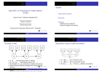
Acoustic Model • P(signal| phones): – Problem: Phones can be pronounced differently • Speaker differences, speaking rate, microphone • Phones may not even appear, different contexts – Observation sequence is uncertain • Solution: Hidden Markov Models – 1) Hidden => Observations uncertain – 2) Probability of word sequences => • State transition probabilities – 3) 1 st order Markov => use 1 prior state

Hidden Markov Models (HMMs) • An HMM is: = Q q q q – 1) A set of states: , ,..., o k 1 = A a a ,..., – 2) A set of transition probabilities: mn 01 • Where aij is the probability of transition qi -> qj B = b i o – 3)Observation probabilities: ( ) t • The probability of observing ot in state i π – 4) An initial probability dist over states: i • The probability of starting in state i – 5) A set of accepting states

Acoustic Model • 3-state phone model for [m] – Use Hidden Markov Model (HMM) 0.3 0.9 0.4 Transition probabilities Onset Mid End Final 0.7 0.1 0.6 C3: C5: C6: C1: C3: C4: C2: C4: C6: 0.3 0.1 0.4 0.5 0.2 0.1 0.2 0.7 0.5 Observation probabilities – Probability of sequence: sum of prob of paths

Viterbi Algorithm • Find BEST word sequence given signal – Best P(words|signal) – Take HMM & VQ sequence • => word seq (prob) • Dynamic programming solution – Record most probable path ending at a state i • Then most probable path from i to end • O(bMn)

Viterbi Code Function Viterbi(observations length T, state-graph) returns best-path Num-states<-num-of-states(state-graph) Create path prob matrix viterbi[num-states+2,T+2] Viterbi[0,0]<- 1.0 For each time step t from 0 to T do for each state s from 0 to num-states do for each transition s’ from s in state-graph new-score<-viterbi[s,t]*at[s,s’]*bs’(ot) if ((viterbi[s’,t+1]=0) || (viterbi[s’,t+1]<new-score)) then viterbi[s’,t+1] <- new-score back-pointer[s’,t+1]<-s Backtrace from highest prob state in final column of viterbi[] & return

Enhanced Decoding • Viterbi problems: – Best phone sequence not necessarily most probable word sequence • E.g. words with many pronunciations less probable – Dynamic programming invariant breaks on trigram • Solution 1: – Multipass decoding: • Phone decoding -> n-best lattice -> rescoring (e.g. tri)

Enhanced Decoding: A* • Search for highest probability path – Use forward algorithm to compute acoustic match – Perform fast match to find next likely words • Tree-structured lexicon matching phone sequence – Estimate path cost: • Current cost + underestimate of total – Store in priority queue – Search best first

Modeling Sound, Redux • Discrete VQ codebook values – Simple, but inadequate – Acoustics highly variable • Gaussian pdfs over continuous values – Assume normally distributed observations • Typically sum over multiple shared Gaussians – “Gaussian mixture models” – Trained with HMM model − 1 1 ′ − µ − µ o o [( ) ( )] = b o e t j t j ∑ j ( ) j t π j ( 2 ) | | ∑

Learning HMMs • Issue: Where do the probabilities come from? • Solution: Learn from data – Trains transition (aij) and emission (bj) probabilities • Typically assume structure – Baum-Welch aka forward-backward algorithm • Iteratively estimate counts of transitions/emitted • Get estimated probabilities by forward comput’n – Divide probability mass over contributing paths

Forward Probability α = = λ i P o o o q j ( ) ( , ,.., , | ) t t t 1 2 α = < < a b o j N ( 1 ) ( ), 1 j j j t 1 − N 1   α = α − t t a b o ( ) ( 1 ) ( ) j ∑ j aj j t   = i  2  − N 1 λ = α = α P O T T a ( | ) ( ) ( ) N ∑ i iN = i 2