Dominators in a Flowgraph Flowgraph: G = ( V, E, r ); each v in V is - PowerPoint PPT Presentation
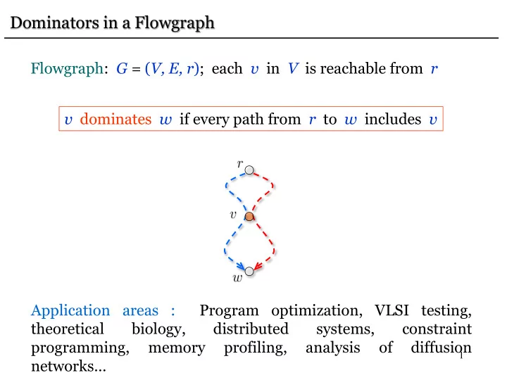
Dominators in a Flowgraph Flowgraph: G = ( V, E, r ); each v in V is reachable from r v dominates w if every path from r to w includes v Application areas : Program optimization, VLSI testing, theoretical biology, distributed systems,
The Lengauer-Tarjan Algorithm: Semidominators • For any w r , idom(w) * sdom(w) + w . • sdom(w) = min ( { v | (v, w) E and v < w } { sdom(u) | u > w and (v, w) E such that u * v } ). sdom(u) sdom(u) nca(w,v) = v nca(w,v) = w nca(w,v) w u w u v v 39
The Lengauer-Tarjan Algorithm: Semidominators • For any w r , idom(w) * sdom(w) + w . • sdom(w) = min ( { v | (v, w) E and v < w } { sdom(u) | u > w and (v, w) E such that u * v } ). • Let w r and let u be any vertex with min sdom(u) that satisfies sdom(w) + u * w . Then idom(w) = idom(u) . sdom(u) sdom(w) idom(w) = idom(u) u w 40
The Lengauer-Tarjan Algorithm: Semidominators • For any w r , idom(w) * sdom(w) + w . • sdom(w) = min ( { v | (v, w) E and v < w } { sdom(u) | u > w and (v, w) E such that u * v } ). • Let w r and let u be any vertex with min sdom(u) that satisfies sdom(w) + u * w . Then idom(w) = idom(u) . Moreover, if sdom(u) = sdom(w) then idom(w) = sdom(w) . sdom(u) = sdom(w) idom(w) = sdom(w) u w 41
The Lengauer-Tarjan Algorithm Overview of the Algorithm 1. Carry out a DFS. 2. Process the vertices in reverse preorder. For vertex w , compute sdom(w) . 3. Implicitly define idom(w) . 4. Explicitly define idom(w) by a preorder pass. 42
Evaluating minima on tree paths sdom(u) sdom(u) nca(w,v) = v nca(w,v) nca(w,v) = w u u w w v v If we process vertices in reverse preorder then the sdom values we need are known. 43
Evaluating minima on tree paths Data Structure: Maintain forest F and supports the operations: link( v , w ): Add the edge (v,w) to F . eval( v ): Let r be the root of the tree that contains v in F . If v = r then return v . Otherwise return any vertex with minimum sdom among the vertices u that satisfy r + u * v . Initially every vertex in V is a root in F . 44
The Lengauer-Tarjan Algorithm dfs( r ) for all w V in reverse preorder do for all v pred(w) do u eval( v ) if semi(u) < semi(w) then semi(w) semi(u) done add w to the bucket of semi(w) link( parent(w) , w ) for all v in the bucket of parent(w) do delete v from the bucket of parent(w) u eval( v ) if semi(u) < semi(v) then dom(v) u else dom(v) parent(w) done done for all w V in reverse preorder do if dom(w) semi(w) then dom(w) dom(dom(w)) 45 done
The Lengauer-Tarjan Algorithm: Example r 1 c 2 b 8 e g 7 3 9 f a 11 10 4 h d 12 j 13 l i 5 k 6 46
The Lengauer-Tarjan Algorithm: Example eval( 12 ) = 12 r 1 c 2 b 8 e g 7 3 9 f a 11 10 4 h d 12 j 13 l i 5 [12] k 6 47
The Lengauer-Tarjan Algorithm: Example add 13 to bucket(12) r 1 link( 13 ) c 2 b 8 e g 7 3 9 f a 11 13 10 4 h d 12 j 13 l i 5 [12] k 6 48
The Lengauer-Tarjan Algorithm: Example delete 13 from bucket(12) r 1 eval(13) = 13 c 2 b 8 e g 7 3 9 f a 11 10 4 h d 12 j 13 l i dom(13)=12 5 [12] k 6 49
The Lengauer-Tarjan Algorithm: Example eval(11) = 11 r 1 c 2 b 8 e g 7 3 9 f a 11 10 4 h d 12 j [11] 13 l i dom(13)=12 5 [12] k 6 50
The Lengauer-Tarjan Algorithm: Example eval(8) = 8 r 1 c 2 b 8 e g 7 3 9 f a 11 10 4 h d 12 j [8] 13 l i dom(13)=12 5 [12] k 6 51
The Lengauer-Tarjan Algorithm: Example add 12 to bucket(8) r 1 link(12) 12 c 2 b 8 e g 7 3 9 f a 11 10 4 h d 12 j [8] 13 l i dom(13)=12 5 [12] k 6 52
The Lengauer-Tarjan Algorithm: Example eval(8)=8 r 1 12 c 2 b 8 e g 7 3 9 f a 11 [8] 10 4 h d 12 j [8] 13 l i dom(13)=12 5 [12] k 6 53
The Lengauer-Tarjan Algorithm: Example eval(1)=1 r 1 12 c 2 b 8 e g 7 3 9 f a 11 [1] 10 4 h d 12 j [8] 13 l i dom(13)=12 5 [12] k 6 54
The Lengauer-Tarjan Algorithm: Example 11 add 11 to bucket(1) r 1 link(11) 12 c 2 b 8 e g 7 3 9 f a 11 [1] 10 4 h d 12 j [8] 13 l i dom(13)=12 5 [12] k 6 55
The Lengauer-Tarjan Algorithm: Example 11 delete 12 from bucket(8) r 1 eval(12) = 11 c 2 b 8 e g 7 3 9 f a 11 [1] 10 4 h d 12 j dom(12)=11 [8] 13 l i dom(13)=12 5 [12] k 6 56
The Lengauer-Tarjan Algorithm: Example 11 eval(13) = 11 r 1 c 2 b 8 e g 7 3 9 f a 11 [1] 10 4 h d 12 j dom(12)=11 [1] [8] 13 l i dom(13)=12 5 [12] k 6 57
The Lengauer-Tarjan Algorithm: Example 11 10 9 8 add 8 to bucket(1) r 1 link(8) c 2 b 8 [1] e g 7 3 9 f a 11 [1] [1] 10 4 h d 12 j dom(12)=11 [1] [8] 13 l i dom(13)=12 5 [12] k 6 58
The Lengauer-Tarjan Algorithm: Example 10 9 8 delete 11 from bucket(1) r 1 eval(11) = 11 c 2 b 8 [1] e g 7 3 9 f a 11 dom(11)=1 [1] [1] 10 4 h d 12 j dom(12)=11 [1] [8] 13 l i dom(13)=12 5 [12] k 6 59
The Lengauer-Tarjan Algorithm: Example 9 8 delete 10 from bucket(1) r 1 eval(10) = 10 c 2 b 8 [1] e g 7 3 9 f a 11 dom(11)=1 [1] [1] 10 4 dom(10)=1 h d 12 j dom(12)=11 [1] [8] 13 l i dom(13)=12 5 [12] k 6 60
The Lengauer-Tarjan Algorithm: Example 8 delete 9 from bucket(1) r 1 eval(9) = 9 c 2 b 8 [1] dom(9)=1 e g 7 3 9 f a 11 dom(11)=1 [1] [1] 10 4 dom(10)=1 h d 12 j dom(12)=11 [1] [8] 13 l i dom(13)=12 5 [12] k 6 61
The Lengauer-Tarjan Algorithm: Example delete 8 from bucket(1) r 1 eval(8) = 8 c 2 b 8 dom(8)=1 [1] dom(9)=1 e g 7 3 9 f a 11 dom(11)=1 [1] [1] 10 4 dom(10)=1 h d 12 j dom(12)=11 [1] [8] 13 l i dom(13)=12 5 [12] k 6 62
The Lengauer-Tarjan Algorithm: Example 6 eval(6) = 6 r 1 c 2 b 8 dom(8)=1 [1] dom(7)=2 dom(9)=1 e g 7 3 9 f a 11 dom(11)=1 [2] [1] [1] 10 4 dom(10)=1 h d 12 j dom(12)=11 [1] [8] 13 l i dom(13)=12 5 [12] [1] k 6 63 [1]
The Lengauer-Tarjan Algorithm: Example 6 5 add 5 to bucket(1) r 1 link(5) c 2 b 8 dom(8)=1 [1] dom(7)=2 dom(9)=1 e g 7 3 9 f a 11 dom(11)=1 [2] [1] [1] 10 4 dom(10)=1 h d 12 j dom(12)=11 [1] [8] 13 l i dom(13)=12 5 [12] [1] k 6 64 [1]
The Lengauer-Tarjan Algorithm: Example 6 5 eval(3) = 3 r 1 c 2 b 8 dom(8)=1 [1] dom(7)=2 dom(9)=1 e g 7 3 9 f a 11 dom(11)=1 [2] [1] [1] 10 4 dom(10)=1 h d 12 j dom(12)=11 [1] [3] [8] 13 l i dom(13)=12 5 [12] [1] k 6 65 [1]
The Lengauer-Tarjan Algorithm: Example 6 5 add 4 to bucket(3) r 1 link(4) c 2 b 8 dom(8)=1 [1] 4 dom(7)=2 dom(9)=1 e g 7 3 9 f a 11 dom(11)=1 [2] [1] [1] 10 4 dom(10)=1 h d 12 j dom(12)=11 [1] [3] [8] 13 l i dom(13)=12 5 [12] [1] k 6 66 [1]
The Lengauer-Tarjan Algorithm: Example 6 5 delete 4 from bucket(3) r 1 eval(4) = 4 c 2 b 8 dom(8)=1 [1] dom(7)=2 dom(9)=1 e g 7 3 9 f a 11 dom(11)=1 [2] [1] [1] 10 4 dom(10)=1 h d 12 j dom(4)=3 dom(12)=11 [1] [3] [8] 13 l i dom(13)=12 5 [12] [1] k 6 67 [1]
The Lengauer-Tarjan Algorithm: Example 6 5 eval(2) = 2 r 1 c 2 b 8 dom(8)=1 [1] dom(7)=2 dom(9)=1 e g 7 3 9 f a 11 dom(11)=1 [2] [1] [2] [1] 10 4 dom(10)=1 h d 12 j dom(4)=3 dom(12)=11 [1] [3] [8] 13 l i dom(13)=12 5 [12] [1] k 6 68 [1]
The Lengauer-Tarjan Algorithm: Example 6 5 eval(5) = 5 r 1 c 2 b 8 dom(8)=1 [1] dom(7)=2 dom(9)=1 e g 7 3 9 f a 11 dom(11)=1 [2] [1] [1] [1] 10 4 dom(10)=1 h d 12 j dom(4)=3 dom(12)=11 [1] [3] [8] 13 l i dom(13)=12 5 [12] [1] k 6 69 [1]
The Lengauer-Tarjan Algorithm: Example 6 5 3 add 3 to bucket(1) r 1 link(3) c 2 b 8 dom(8)=1 [1] dom(7)=2 dom(9)=1 e g 7 3 9 f a 11 dom(11)=1 [2] [1] [1] [1] 10 4 dom(10)=1 h d 12 j dom(4)=3 dom(12)=11 [1] [3] [8] 13 l i dom(13)=12 5 [12] [1] k 6 70 [1]
The Lengauer-Tarjan Algorithm: Example 6 5 3 eval(1) = 1 r 1 c 2 [1] b 8 dom(8)=1 [1] dom(7)=2 dom(9)=1 e g 7 3 9 f a 11 dom(11)=1 [2] [1] [1] [1] 10 4 dom(10)=1 h d 12 j dom(4)=3 dom(12)=11 [1] [3] [8] 13 l i dom(13)=12 5 [12] [1] k 6 71 [1]
The Lengauer-Tarjan Algorithm: Example 6 5 3 2 add 2 to bucket(1) r 1 link(2) c 2 [1] b 8 dom(8)=1 [1] dom(7)=2 dom(9)=1 e g 7 3 9 f a 11 dom(11)=1 [2] [1] [1] [1] 10 4 dom(10)=1 h d 12 j dom(4)=3 dom(12)=11 [1] [3] [8] 13 l i dom(13)=12 5 [12] [1] k 6 72 [1]
The Lengauer-Tarjan Algorithm: Example 5 3 2 delete 6 from bucket(1) r 1 eval(6) = 6 c 2 [1] b 8 dom(8)=1 [1] dom(7)=2 dom(9)=1 e g 7 3 9 f a 11 dom(11)=1 [2] [1] [1] [1] 10 4 dom(10)=1 h d 12 j dom(4)=3 dom(12)=11 [1] [3] [8] 13 l i dom(13)=12 5 [12] [1] dom(6)=1 k 6 73 [1]
The Lengauer-Tarjan Algorithm: Example 3 2 delete 5 from bucket(1) r 1 eval(5) = 5 c 2 [1] b 8 dom(8)=1 [1] dom(7)=2 dom(9)=1 e g 7 3 9 f a 11 dom(11)=1 [2] [1] [1] [1] 10 4 dom(10)=1 h d 12 j dom(4)=3 dom(12)=11 [1] [3] [8] 13 l i dom(13)=12 5 dom(5)=1 [12] [1] dom(6)=1 k 6 74 [1]
The Lengauer-Tarjan Algorithm: Example 2 delete 3 from bucket(1) r 1 eval(3) = 3 c 2 [1] b 8 dom(8)=1 [1] dom(7)=2 dom(9)=1 e g 7 3 9 f dom(3)=1 a 11 dom(11)=1 [2] [1] [1] [1] 10 4 dom(10)=1 h d 12 j dom(4)=3 dom(12)=11 [1] [3] [8] 13 l i dom(13)=12 5 dom(5)=1 [12] [1] dom(6)=1 k 6 75 [1]
The Lengauer-Tarjan Algorithm: Example delete 2 from bucket(1) r 1 eval(2) = 2 c 2 [1] b dom(2)=1 8 dom(8)=1 [1] dom(7)=2 dom(9)=1 e g 7 3 9 f dom(3)=1 a 11 dom(11)=1 [2] [1] [1] [1] 10 4 dom(10)=1 h d 12 j dom(4)=3 dom(12)=11 [1] [3] [8] 13 l i dom(13)=12 5 dom(5)=1 [12] [1] dom(6)=1 k 6 76 [1]
The Lengauer-Tarjan Algorithm: Example dom(12) semi(12) r 1 set dom(12)=dom(11) c 2 [1] b dom(2)=1 8 dom(8)=1 [1] dom(7)=2 dom(9)=1 e g 7 3 9 f dom(3)=1 a 11 dom(11)=1 [2] [1] [1] [1] 10 4 dom(10)=1 h d 12 j dom(4)=3 dom(12)=1 [1] [3] [8] 13 l i dom(13)=12 5 dom(5)=1 [12] [1] dom(6)=1 k 6 77 [1]
The Lengauer-Tarjan Algorithm Running Time = O(n + m) + Time for n -1 calls to link() + Time for m + n -1 calls to eval() 78
Data Structure for link() and eval() We want to apply Path Compression : v 0 [ l 0 ] v 0 [ l 0 ] eval( v 3 ) v 1 [ l 1 ] v 2 [ l 2 ] v 3 [ l’ 3 ] v 2 [ l’ 2 ] v 1 [ l’ 1 ] v 3 [ l 3 ] l’ 1 = l 1 semi(l’ 2 ) = min { semi(l 1 ) , semi(l 2 ) } semi(l’ 3 ) = min { semi(l 1 ) , semi(l 2 ) , semi(l 3 ) } 79
Data Structure for link() and eval() We maintain a virtual forest VF such that: 1. For each T in F there is a corresponding VT in VF with the same vertices as T . 2. Corresponding trees T and VT have the same root with the same label. 3. If v is any vertex, eval( v , F ) = eval( v , VF ). Representation: ancestor(v) = parent of v in VT . 80
Data Structure for link() and eval() eval( v ): Compress the path r * v and return the label of v . link( v , w ): Make v the parent of w . VF satisfies Properties 1-3. Time for n -1 calls to link() + Time for m + n -1 calls to eval() = O(m log 2+ m / n n) 81
Experimental Results (Small Graphs) 82
Experimental Results (Large Graphs) 83 Running time in ms . Missing values correspond to execution time >1 h.
The Lengauer-Tarjan Algorithm: Correctness Lemma 1: v , w such that v w , any path from v to w contains a common ancestor of v and w in T . Follows from Property 1 Lemma 2: For any w r , idom(w) is an ancestor of w in T . idom(w) is contained in every path from r to w 84
The Lengauer-Tarjan Algorithm: Correctness Lemma 3: For any w r , sdom(w) is an ancestor of w in T . • (parent(w), w) is an SDOM-path sdom(w) parent(w) . • SDOM-path P = ( v 0 = sdom(w) , v 1 , …, v k = w ); Lemma 1 some v i is a common ancestor of sdom(w) and w . We must have v i sdom(w) v i = sdom(w) . 85
The Lengauer-Tarjan Algorithm: Correctness Lemma 4: For any w r , idom(w) is an ancestor of sdom(w) in T . sdom(w) The SDOM-path from sdom(w) to w avoids the proper ancestors of w that SDOM-path are proper descendants of sdom(w) . w 86
The Lengauer-Tarjan Algorithm: Correctness Lemma 5: Let v , w satisfy v * w . Then v * idom(w) or idom(w) * idom(v) . For each x that satisfies idom(v) idom(v) + x + v x there is a path P x from r to v that avoids x . idom(w) P x P x v * w is a path from r to w that avoids x idom(w) x . v 87 w
The Lengauer-Tarjan Algorithm: Correctness Theorem 2: Let w r . If sdom(u) sdom(w) for every u that satisfies sdom(w) + u * w then idom(w) = sdom(w) . r Suppose for contradiction sdom(w) Dom(w) path P from r to w that x avoids sdom(w) . sdom(w) P x = last vertex P such that x < sdom(w) y = first vertex P sdom(w) * w y Q = part of P from x to y w Lemma 1 y < u , u Q – { x , y } sdom(y) < sdom(w) . 88
The Lengauer-Tarjan Algorithm: Correctness Theorem 3: Let w r and let u be any vertex for which sdom(u) is minimum among the vertices u that satisfy sdom(w) + u * w . Then idom(u) = idom(w) . r x Lemma 4 and Lemma 5 idom(w) * idom(u) . P idom(u) Suppose for contradiction idom(u) idom(w) . y path P from r to w that avoids idom(u) . sdom(w) u 89 w
The Lengauer-Tarjan Algorithm: Correctness Theorem 3: Let w r and let u be any vertex for which sdom(u) is minimum among the vertices u that satisfy sdom(w) + u * w . Then idom(u) = idom(w) . r x = last vertex P such that x < idom(u) . x y = first vertex P idom(u) * w . P idom(u) Q = part of P from x to y . Lemma 1 y < u , u Q – { x , y } y sdom(y) < idom(u) sdom(u) . sdom(w) Therefore y v for any v that satisfies u idom(u) + v * u . 90 But y cannot be an ancestor of idom(u) . w
The Lengauer-Tarjan Algorithm: Correctness From Theorem 2 and Theorem 3 we have sdom idom : Corollary 1: Let w r and let u be any vertex for which sdom(u) is minimum among the vertices u that satisfy sdom(w) + u * w . Then idom(w) = sdom(w) , if sdom(w) = sdom(w) and idom(w) = idom(u) otherwise. We still need a method to compute sdom . 91
The Lengauer-Tarjan Algorithm: Correctness Theorem 4: For any w r , sdom(w) = min ( { v | ( v , w ) E and v < w } { sdom(u) | u > w and ( v , w ) E such that u * v } ). Let x = min ( { v | ( v , w ) E and v < w } { sdom(u) | u > w and ( v , w ) E such that u * v } ). We first show sdom(w) x and then sdom(w) x . 92
The Lengauer-Tarjan Algorithm: Correctness Theorem 4: For any w r , sdom(w) = min ( { v | ( v , w ) E and v < w } { sdom(u) | u > w and ( v , w ) E such that u * v } ). • sdom(w) x Assume x = v such that ( v , w ) E and v < w sdom(w) x . 93
The Lengauer-Tarjan Algorithm: Correctness Theorem 4: For any w r , sdom(w) = min ( { v | ( v , w ) E and v < w } { sdom(u) | u > w and ( v , w ) E such that u * v } ). • sdom(w) x Assume x = sdom(u) such that u > w and ( v , w ) E for some x = sdom(u) descendant v of u in T . P P = SDOM-path from x to u u P u * v ( v , w ) is an SDOM-path from x to w . w v 94
The Lengauer-Tarjan Algorithm: Correctness Theorem 4: For any w r , sdom(w) = min ( { v | ( v , w ) E and v < w } { sdom(u) | u > w and ( v , w ) E such that u * v } ). • sdom(w) x Assume that ( sdom(w) , w ) E sdom(w) x . 95
The Lengauer-Tarjan Algorithm: Correctness Theorem 4: For any w r , sdom(w) = min ( { v | ( v , w ) E and v < w } { sdom(u) | u > w and ( v , w ) E such that u * v } ). • sdom(w) x Assume that P = ( sdom(w) = v 0 , v 1 , … , v k = w ) is a simple path v i > w , 1 i k -1. sdom(w) P j = min { i 1 | v i * v k-1 }. w v j Lemma 1 v i > v j , 1 i j -1 x sdom(v j ) sdom(w) . 96 v k-1
The Lengauer-Tarjan Algorithm: Almost-Linear-Time Version We get better running time if the trees in F are balanced (as in Set-Union). F is balanced for constants a > 1, c > 0 if for all i we have: # vertices in F of height i cn/a i Theorem 5 [Tarjan 1975]: The total length of an arbitrary sequence of m path compressions in an n -vertex forest balanced for a , c is O((m+n) (m+n, n)) , where the constant depends on a and c . 97
Linear-Time Algorithms There are linear-time dominators algorithms both for the RAM Model and the Pointer-Machine Model. • Based on LT, but much more complicated. • First published algorithms that claimed linear-time , in fact didn’t achieve that bound. RAM: Harel [1985] Alstrup, Harel, Lauridsen and Thorup [1999] Pointer-Machine: Buchsbaum, Kaplan, Rogers and Westbrook [1998] G. and Tarjan [2004], 98 Buchsbaum, G., Kaplan, Rogers, Tarjan and Westbrook [2008]
GT Linear-Time Algorithm: High-Level View Partition DFS-tree D into nontrivial microtrees and lines. Nontrivial microtree: Maximal subtree of D of size g that contains at least one leaf of D . Trivial microtree: Single internal vertex of D . Line: Maximal unary path of 1 trivial microtrees. lines 2 16 3 17 20 27 30 4 5 6 13 18 19 21 28 29 31 7 14 15 22 8 9 23 24 nontrivial 10 25 g =3 microtrees 99 11 12 26
GT Linear-Time Algorithm: High-Level View Partition DFS-tree D into nontrivial microtrees and lines. Nontrivial microtree: Maximal subtree of D of size g that contains at least one leaf of D . Trivial microtree: Single internal vertex of D . Line: Maximal unary path of 1 trivial microtrees. 2 16 {1} Core C : Tree D – nontrivial microtrees 3 20 {2,3,6,7,9} {16,20,21,22} 6 21 C’ : contract each line of C to C’ a sigle vertex 7 22 9 C 100
Recommend
More recommend
Explore More Topics
Stay informed with curated content and fresh updates.
