Control-Flow Analysis and Loop Detection Last time PRE Today - PDF document

Control-Flow Analysis and Loop Detection � Last time – � PRE � Today – � Control-flow analysis – � Loops – � Identifying loops using dominators – � Reducibility – � Using loop identification to identify induction variables � CS553 Lecture Control-Flow and Loop Detection 1 Context � Data-flow – � Flow of data values from defs to uses – � Could alternatively be represented as a data dependence � Control-flow – � Sequencing of operations – � Could alternatively be represented as a control dependence – � e.g., Evaluation of then-code and else-code depends on if-test CS553 Lecture Control-Flow and Loop Detection 2

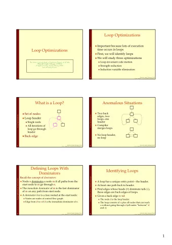
Why study control flow analysis? � Finding Loops – � most computation time is spent in loops – � to optimize them, we need to find them � Loop Optimizations – � Loop-invariant code hoisting – � Induction variable elimination – � Array bounds check removal – � Loop unrolling – � Parallelization – � ... � Identifying structured control flow – � can be used to speed up data-flow analysis CS553 Lecture Control-Flow and Loop Detection 3 Representing Control-Flow � High-level representation – � Control flow is implicit in an AST � Low-level representation: – � Use a Control-flow graph – � Nodes represent statements – � Edges represent explicit flow of control � Other options – � Control dependences in program dependence graph (PDG) [Ferrante87] – � Dependences on explicit state in value dependence graph (VDG) [Weise 94] CS553 Lecture Control-Flow and Loop Detection 4

What Is Control-Flow Analysis? � Control-flow analysis discovers the flow of control within a procedure ( e.g., builds a CFG, identifies loops) 1 a := 0 � Example b := a * b � 1 a := 0 3 c := b/d � 2 b := a * b c < x? � 3 L1: c := b/d � 4 if c < x goto L2 5 e := b / c � 5 e := b / c f := e + 1 � 6 f := e + 1 � 7 L2: g := f 7 g := f � 8 h := t - g h := t - g � 9 if e > 0 goto L3 e > 0? � 10 goto L1 No Yes � 11 L3: return goto return 10 11 CS553 Lecture Control-Flow and Loop Detection 5 Loop Concepts � Loop : Strongly connected subgraph of CFG with a single entry point (header) � Loop entry edge : Source not in loop & target in loop � Loop exit edge : Source in loop & target not in loop � Loop header node : Target of loop entry edge. Dominates all nodes in loop. � Back edge : Target is loop header & source is in the loop � Natural loop : Associated with each back edge. Nodes dominated by header and with path to back edge without going through header � Loop tail node : Source of back edge � Loop preheader node : Single node that’s source of the loop entry edge � Nested loop : Loop whose header is inside another loop CS553 Lecture Control-Flow and Loop Detection 6

Picturing Loop Terminology preheader back edge entry edge head loop tail exit edge CS553 Lecture Control-Flow and Loop Detection 7 The Value of Preheader Nodes � Not all loops have preheaders h – � Sometimes it is useful to create them � Without preheader node t – � There can be multiple entry edges pre-header p � With single preheader node – � There is only one entry edge h � Useful when moving code outside the loop t – � Don’t have to replicate code for multiple entry edges CS553 Lecture Control-Flow and Loop Detection 8

Identifying Loops � Why? – � Most execution time spent in loops, so optimizing loops will often give most benefit � Many approaches – � Interval analysis – � Exploit the natural hierarchical structure of programs – � Decompose the program into nested regions called intervals – � Structural analysis: a generalization of interval analysis – � Identify dominators to discover loops � We’ll focus on the dominator-based approach CS553 Lecture Control-Flow and Loop Detection 9 Dominator Terminology entry Dominators d dom i if all paths from entry to node i include d d dom i d Strict dominators d sdom i if d dom i and d � i entry � i Immediate dominators a a idom b a idom b if a sdom b and there does not exist a node c � such that c � a, c � b, a dom c, and c dom b not � c, a sdom c and c sdom b b Post dominators i p pdom i if every possible path from i to exit includes � p (p dom i in the flow graph whose arcs are reversed and entry and exit are interchanged) p pdom i p exit CS553 Lecture Control-Flow and Loop Detection 10

Identifying Natural Loops with Dominators t Back edges A back edge of a natural loop is one whose target back edge dominates its source s Natural loop The natural loop of a back edge (m � n), where n n dominates m, is the set of nodes x such that n natural dominates x and there is a path from x to m not loop containing n m a a The target, c, of the b Example edge (d � c) does not b SCC with c and d not c dominate its source, d, a loop because has so (d � c) does not c d d two entry points define a natural loop e e CS553 Lecture Control-Flow and Loop Detection 11 Computing Dominators Input : Set of nodes N (in CFG) and an entry node s Output : Dom[i] = set of all nodes that dominate node i Dom[s] = {s} Key Idea for each n � N – {s} If a node dominates all Dom[n] = N predecessors of node n, then it also dominates node n repeat change = false for each n � N – {s} p 2 p 1 p 3 pred[n] D = {n} � ( � p � pred(n) Dom[p]) if D � Dom[n] n change = true Dom[n] = D until !change x � Dom(p 1 ) ^ x � Dom(p 2 ) ^ x � Dom(p 3 ) � x � Dom(n) CS553 Lecture Control-Flow and Loop Detection 12

Computing Dominators (example) Input : Set of nodes N and an entry node s Output : Dom[i] = set of all nodes that dominate node i s {s} {n, p, q, r, s} q {n, p, q, r, s} {n, p, q, r, s} {n, p, q, r, s} r Dom[s] = {s} for each n � N – {s} p {n, p, q, r, s} {n, p, q, r, s} Dom[n] = N n {n, p, q, r, s} {n, p, q, r, s} repeat Initially change = false Dom[s] = {s} for each n � N – {s} Dom[q] = {n, p, q, r, s} . . . D = {n} � ( � p � pred(n) Dom[p]) Finally if D � Dom[n] Dom[q] = {q, s} change = true Dom[r] = {r, s} Dom[n] = D until !change Dom[p] = {p, s} Dom[n] = {n, p, s} CS553 Lecture Control-Flow and Loop Detection 13 Reducibility � Definitions – � A CFG is reducible (well-structured) if we can partition its edges into two disjoint sets, the forward edges and the back edges, such that – � The forward edges form an acyclic graph in which every node can be reached from the entry node – � The back edges consist only of edges whose targets dominate their sources – � A CFG is reducible if it can be converted into a single node using T1 and T2 transformations. � Structured control-flow constructs give rise to reducible CFGs � Value of reducibility – � Dominance useful in identifying loops – � Simplifies code transformations (every loop has a single header) – � Permits interval analysis and it is easy to calculate the CFG depth CS553 Lecture Control-Flow and Loop Detection 14

T1 and T2 transformations � T1 transformation a a – � remove self-cycles � T2 transformation – � if node n has a unique predecessor p, then remove n and make all the successors for n be successors for p a ab b c d c d CS553 Lecture Control-Flow and Loop Detection 15 Handling Irreducible CFG’s � Node splitting – � Can turn irreducible CFGs into reducible CFGs a a b b c d c d e e d �� e �� CS553 Lecture Control-Flow and Loop Detection 16

Why Go To All This Trouble? � Modern languages provide structured control flow – � Shouldn’t the compiler remember this information rather than throw it away and then re-compute it? � Answers? – � We may want to work on the binary code in which case such information is unavailable – � Most modern languages still provide a goto statement – � Languages typically provide multiple types of loops. This analysis lets us treat them all uniformly – � We may want a compiler with multiple front ends for multiple languages; rather than translate each language to a CFG, translate each language to a canonical LIR, and translate that representation once to a CFG CS553 Lecture Control-Flow and Loop Detection 17 Induction variables � Induction variable identification – � Induction variables – � Variables whose values form an arithmetic progression � Why bother? – � Useful for strength reduction, induction variable elimination, loop transformations, and automatic parallelization � Simple approach – � Search for statements of the form, i = i + c – � Examine reaching definitions to make sure there are no other defs of i in the loop – � Does not catch all induction variables. Examples? CS553 Lecture Induction Variables 18

Example Induction Variables � s = 0; � for (i=0; i<N; i++) � s += a[i]; CS553 Lecture Induction Variables 19 Induction Variable Identification � Types of Induction Variables – � Basic induction variables (eg. loop index) – � Variables that are defined once in a loop by a statement of the form, i=i+c (or i=i-c ), where c is a constant integer or loop invariant – � Derived induction variables – � Variables that are defined once in a loop as a linear function of another induction variable – � k = j + c 1 or – � k = c 2 * j where c 1 and c 2 are loop invariant CS553 Lecture Induction Variables 20