CO444H SSA SSA Construction SSA-based analysis Ben Livshits 1 - PowerPoint PPT Presentation
Dataflow Solutions CO444H SSA SSA Construction SSA-based analysis Ben Livshits 1 Refresher: Reaching Definitions Direction D = forward. Domain V = set of all sets of definitions in the flow graph. = union. Functions F =
Dataflow Solutions CO444H SSA SSA Construction SSA-based analysis Ben Livshits 1
Refresher: Reaching Definitions • Direction D = forward. • Domain V = set of all sets of definitions in the flow graph. • ∧ = union. • Functions F = all “gen - kill” functions of the form f(x) = (x - KILL) ∪ GEN, where KILL and GEN are sets of definitions (members of V). 2
Last Time: May vs. Must Analysis May Must Forward Reaching Available definitions expressions Backward Live variables Very busy expressions 3
4 Different Dataflow Solutions
What Does the Iterative Algorithm Do? • IDEAL = ideal solution = meet over all executable paths from entry to a point • MOP = meet over all paths from entry to a given point, of the transfer function along that path applied to v ENTRY • MFP ( maximal fixedpoint ) = result obtained by running the iterative algorithm from last lecture 5
Transfer Function of a Path . . . f 1 f 2 f n-1 B f n-1 ( . . .f 2 (f 1 (v ENTRY )). . .) 6
Maximum Fixedpoint • Fixedpoint = solution to the equations used in iteration: IN(B) = ∧ predecessors P of B OUT(P); OUT(B) = f B (IN(B)); 7
Why Maximum? Maximum = any other solution is ≤ the result of the iterative algorithm (MFP) 8
MOP and IDEAL • All solutions are really meets of the result of starting with v ENTRY and following some set of paths to the point in question • If we don’t include at least the IDEAL paths, we have an error – we are not conservative • But try not to include too many more – try to be precise 9
MOP Versus IDEAL --- (1) • At each block B, MOP[B] ≤ IDEAL[B]. • i.e., the meet over many paths is ≤ the meet over a subset. • Example: • x ∧ y ∧ z ≤ x ∧ y • because x ∧ y ∧ z ∧ x ∧ y = x ∧ y ∧ z. • Intuition: Anything not ≤ IDEAL is not safe, because there is some executable path whose effect is not accounted for. 10
MOP Versus IDEAL --- (2) • Conversely: any solution that is ≤ IDEAL accounts for all executable paths (and maybe more paths), and is therefore conservative (safe), even if not accurate. 11
MFP Versus MOP --- (1) • Is MFP ≤ MOP? • If so, then since MOP ≤ IDEAL, we have MFP ≤ IDEAL, and therefore MFP is safe. • Yes, but … requires two important assumptions about the framework: 1. “Monotonicity” 2. Finite height (no infinite chains . . . < x 2 < x 1 < x within the lattice) 12
MFP Versus MOP --- (2) • Intuition: If we computed the MOP directly, we would compose functions along all paths, then take a big meet • But the MFP (iterative algorithm) alternates compositions and meets somewhat arbitrarily • Also, meets occur early, which causes a loss of precision 13
Monotonicity • A framework is monotone if the transfer function (call it f) respects ≤ . • That is: • If x ≤ y, then f(x) ≤ f(y). • Equivalently: f(x ∧ y) ≤ f(x) ∧ f(y). • Intuition: it is conservative to take a meet before completing the composition of functions. 14
Motonotonicity is Quite Common • The frameworks we’ve studied so far are all monotone: • Easy to prove for functions in GEN/KILL form • Try proving this yourself for reaching definitions, for example • And they all are finite height • Only a finite number of definitions, variables, etc. in any given program • You can only iterate so many times 15
Two Paths to B That Meet Early MOP considers paths f(x) independently and In MFP, Values x and y and combines at get combined too soon. the last possible OUT = x moment. f OUT = f(x) ∧ f(y) IN = x ∧ y B ENTRY OUT = f(x ∧ y) OUT = y f(y) Since f(x ∧ y) ≤ f(x) ∧ f(y), we might have lost some precision because of the early meet 16
Distributive Frameworks • Strictly stronger than monotonicity is the distributivity condition: f(x ∧ y) = f(x) ∧ f(y) • Functions F = all “gen - kill” functions of the form f(x) = (x - KILL) ∪ GEN, where KILL and GEN are sets of definitions (members of V) (x – (K1 U K2)) U (G1UG2) = (x-K1) U G1 U (x-K2) U G2 17
Advantages of Distributivity • All the GEN/KILL frameworks are distributive. • If a framework is distributive, then combining paths early doesn’t hurt. • MOP = MFP • That is, the iterative algorithm computes a solution that takes into account all and only the physical paths. • It also does so quite fast 18
19 What Are Some of the Disadvantages of Multiple Reaching Definitions
20 SSA SSA Representation SSA Construction Analysis based on SSA
Static Single Assignment • Each variable has only one reaching definition • When two definitions of the same variable merge, a Ф function is introduced, with a new definition of the variable • First consider SSA for alias-free variables 21
Example: CFG a = a = = a+5 = a+5 a = Multiple reaching definitions = a+5 22
Example: SSA Form a 3 = a 1 = = a 1 +5 a 4 = Ф (a 1 ,a 3 ) a 2 = = a 4 +5 = a 2 +5 Single reaching definition 23
Ф Functions • A Ф operand represents the reaching definition from the corresponding predecessor • The ordering of Ф operands are important for knowing from which path the definition is coming from • The predicate is generally not recorded as part of the Ф function 24
SSA Conditions 1. If • two non-null paths X → + Z and Y → + Z converge at node Z, and • nodes X and Y contains (V =..), • then V = Ф (V, .., V) has been inserted at Z 2. Each mention of V has been replaced by a mention of V i 3. V and the corresponding V i have the same value. 25
26 SSA Placement SSA Representation SSA Construction Step 1: Place Ф statements Step 2: Rename all variables Converting out of SSA
Ф Function Placement Place a = … minimal number of a = Ф (a ,a) Ф functions a = Ф (a ,a) 27
Renaming Uses to Refer to Proper Definitions a 2 = a 1 = a 1 +5 a 3 = Ф (a 1 ,a 2 ) a 4 = a 4 +5 a 3 +5 28
SSA Construction Algorithm (I) • Step 1: Place Ф statements by computing iterated dominance frontier 29
Control Flow Graph (CFG) • A control flow graph G = (V, E) • Set V contains distinguished nodes START and END • Every node is reachable from START • END is reachable from every node in G. • START has no predecessors • END has no successors. • Predecessor, successor, path 30
Dominator Relation • If X appears on every path from START to Y, then X dominates Y • Domination is both reflexive and transitive • IDOM(Y): immediate dominator of Y • Dominator Tree • START is the root • Any node Y other than START has IDOM(Y) as its parent • Parent, child, ancestor, descendant 31
Dominator Tree Example START START a c b d CFG DT END 32
Dominator Tree Example START START a a c b d CFG DT END 33
Dominator Tree Example START START a a c b b c d CFG DT END 34
Dominator Tree Example START START a a c b b d c d CFG DT END 35
Dominator Tree Example START START a END a c b b d c d CFG DT END 36
Dominance Frontier • Dominance frontier DF(X) for node X is a set of nodes Y such that 1. X dominates a predecessor of Y 2. X does not strictly dominate Y 37
DF Example START START a END a c b b d c DT d DF(c) = ? DF(a) = ? CFG END 38
DF Example START START a END a c b b d c DT d DF(c) = {d} DF(a) = ? CFG END 39
DF Example START START a END a c b b d c DT d DF(c) = {d} DF(a) = {END} CFG END 40
Computing DF(X) START • DF(X) is the union of the following sets • DF local (X), a set of successor a nodes that X doesn’t strictly dominate • E.g. DF local (c) = {d}, see previous slide c b • DF up (Z) for all Z є Children(X) • DF up (Z) = {Y є DF(Z) such that IDOM(Z) doesn’t d strictly dominate Y} • E.g. X = a, Z = d, Y = END, see previous slide END 41
Iterated Dominance Frontier • We can also define this notion for sets of nodes: DF(SET) is the union of DF(X), where X є SET. • Iterated dominance frontier DF + (SET) is the limit of • DF 1 = DF(SET) and DF i+1 = DF(SET U DF i ) 42
Computing Joins • J(SET) of join nodes • Set of all nodes Z • There are (at least) two non-null CFG paths that start at two distinct nodes in SET and converge at Z • Iterated join J + (SET) is the limit of • J 1 = J(SET) and J i+1 = J(SET U J i ) • J + (SET) = DF + (SET) 43
Placement of Ф Functions in SSA • for each variable V • add all nodes with assignments to V to worklist W • for-each X in worklist W do • for-each Y in DF(X) do • if no Ф added in Y then • place (V = Ф (V,…,V)) at Y • if Y has not been added before, add Y to W. 44
Computational Complexity S a • Constructing SSA takes O(A tot * avrgDF), where b • A tot : total number of assignments • avrgDF: weighted average DF size c • The computational complexity is O(n 2 ). d • e.g. nested repeat-until loops E 45
Ф Placement Example a = … Place Ф at Iterative Dominance a = Ф (a ,a) Frontiers a = Ф (a ,a) 46
SSA Construction (II) • Step 2: Rename all variables in original program and Ф functions, using dominator tree and renaming stack to keep track of the current names. 47
Recommend
More recommend
Explore More Topics
Stay informed with curated content and fresh updates.


