Decision Making Marco Chiarandini Department of Mathematics & - PowerPoint PPT Presentation
DM842 Computer Game Programming: AI Lecture 6 Decision Making Marco Chiarandini Department of Mathematics & Computer Science University of Southern Denmark Outline 1. Other Ideas 2. Decision Making Decision Trees 3. State Machine 4.
DM842 Computer Game Programming: AI Lecture 6 Decision Making Marco Chiarandini Department of Mathematics & Computer Science University of Southern Denmark
Outline 1. Other Ideas 2. Decision Making Decision Trees 3. State Machine 4. Behavior Trees 2
Outline 1. Other Ideas 2. Decision Making Decision Trees 3. State Machine 4. Behavior Trees 3
Open Goal Pathfinding check if a node is a goal heuristics need to report the distance to the nearest goal. This is problematic and handled by decision making (selecting a goal). 4
Dynamic Pathfinding environment is changing in unpredictable ways or its information is incomplete. replan each time new information is collected replan only the part that has changed � D ∗ but requires a lot of storage space for, eg, storing path estimates and the parents of nodes in the open list 5
Memory-Bounded Search Try to reduce memory needs Take advantage of heuristic to improve performance Iterative-deepening A ∗ (IDA ∗ ) SMA ∗ 6
Iterative Deepening A ∗ IDA ∗ Idea from classical Uniformed Iterative Deepening depth-first search where the max depth is iteratively increased skip open and closed list depth-first search with cutoff on the f -cost cutoff set on the smallest f -cost of nodes that exceeded the threshold at the previous iteration very simple to implement but less efficient is the "best" variant for goal-oriented action planning in decision making 7
Properties of IDA ∗ Complete Yes Time complexity Still exponential Space complexity linear Optimal Yes. Also optimal in the absence of monotonicity 8
Simple Memory-Bounded A ∗ Use all available memory Follow A ∗ algorithm and fill memory with new expanded nodes If new node does not fit remove stored node with worst f -value propagate f -value of removed node to parent SMA ∗ will regenerate a subtree only when it is needed the path through subtree is unknown, but cost is known 9
Properties of SMA ∗ Complete yes, if there is enough memory for the shortest solution path Time same as A ∗ if enough memory to store the tree Space use available memory Optimal yes, if enough memory to store the best solution path In practice, often better than A ∗ and IDA ∗ trade-off between time and space requirements 10
Recursive Best First Search (a) After expanding Arad, Sibiu, ∞ Arad and Rimnicu Vilcea 366 447 Sibiu Timisoara Zerind 393 447 449 415 Arad Fagaras Oradea Rimnicu Vilcea 413 671 646 415 Craiova Pitesti Sibiu 553 526 417 (b) After unwinding back to Sibiu ∞ and expanding Fagaras Arad 366 447 Sibiu Timisoara Zerind 393 447 449 417 Arad Fagaras Oradea Rimnicu Vilcea 671 646 415 413 417 Sibiu Bucharest 591 450 (c) After switching back to Rimnicu Vilcea ∞ and expanding Pitesti Arad 366 447 Sibiu Timisoara Zerind 393 447 449 447 Arad Fagaras Oradea Rimnicu Vilcea 417 646 415 450 671 447 Craiova Pitesti Sibiu 526 417 553 Bucharest Craiova Rimnicu Vilcea 418 615 607 11
Recursive Best First Search 12
Other Issues Interruptible Pathfinding rendering needs to run every 1/60 or 1/30 of a second ( = 0 . 6 ms ) A* algorithm can be easily stopped and resumed. data required to resume are all contained in the open and closed lists. In Real Time Strategy games: possible many requests to pathfinding at the same time serial � problems for time, parallel � problems for space central pool of pathfinding + path finding queue (FIFO). information from previous pathfinding runs could be useful to be stored above all valid for hierarchical pathfinding) 13
Continuous Pathfinding Vehicle pathfinding: eg, police car pursuing a criminal Split down by placing a node every few yards along the road path = a period of time in a sequence of adjacent lanes. But cars are moving. Depending on the speed the gap may be there or not. A ∗ in a graph where nodes represent states rather than positions a node has two elements: a position and a time. an edge exists between two nodes if the end node can be reached from the start node and if the time it takes to reach the node is correct. two different nodes may represent the same position 14
graph created dynamically: connections, so they are built from scratch when the outgoing connections are requested from the graph. retrieving the out-going connections from a node is a very time-consuming process � avoid A ∗ versions that need recalculations It should be used for only small sections of planning. Eg, plan a route for only the next 100 yards or so. The remainder of the route planned on intersection-by-intersection basis. The pathfinding system that drove the car was hierarchical, with the continuous planner being the lowest level of the hierarchy. 15
Movement Planning If characters are highly constrained, then the steering behaviors might not produce sensible results. Eg: urban driving. Chars have, eg, walk animation, run animation, or sprint animation Animations need specific conditions for being believable plan sequence of animations to reach a large scale maneuver 16
Movement planning uses a graph representation. Each node of the graph represents both the position and the state of the character at that point, ie, the velocity vector, that determines the set of allowable animations that can follow Connections in the graph represent valid animations; lead to nodes representing the char after the animation route returned consists of a set of animations If the velocities and positions are continuous, then infinite number of possible connections. Heuristic only returns the best successor nodes for addition to the open list. similarly to continuous pathfinding, graph is generated on the fly and recomputations in A ∗ are avoided. 17
Example Walking bipedal character Animations: walk, stand to walk, walk to stand, sidestep, and turn on the spot. They can be applied to a range of movement distances Positions: Each animation starts or ends from one of two positions: mid-walk or standing still. Some positions in the environment are forbidden State machine: positions ≡ states and transitions ≡ animations. Goal: range of positions with no orientation. 18
Result from A ∗ : 19
Outline 1. Other Ideas 2. Decision Making Decision Trees 3. State Machine 4. Behavior Trees 20
Decision Making Decision Making: ability of a character to decide what to do. We saw already how to carry out that decision (movement, animation, ...). From animation control to complex strategic and tactical AI. state machines, decision trees rule-based systems fuzzy logic neural networks 21
Input internal and external knowledge Output action Knowledge representation: External knowledge identical for all algorithms Message passing system. Eg, danger is a constant at the character. Every new object in toolchain needs to define when to send message danger and the character will react. Internal knowledge algorithm dependent Actions: Objects notify which actions they are capable of by means of flags. For goal oriented behavior, every action has a list of goals that will be achieved Alternatively, actions as objects with associated data such as state of world after action, animations, etc. Actions are then associated to objects. 22
The Toolchain AI-related elements of a complete toolchain Custom-designed level editing tools to be reused over all the games data driven or object oriented. Each object in the game world has a set of data associated with it that controls behavior Eg, data type “to be avoided” / “to be collected”. Different characters require different decision making logic and behavior Allowing level designers to have access to the AI of characters they are placing without a programmer requires specialist AI design tools. Eg: AI-Implant and SimBionic provide a palette of AI behaviour to combine Actions selected by level designer are mostly steering behaviors. They are put together by the graphical definition of finite state machines Debugging at run time SDK that allows new functionality to be implemented in the form of plug-in tools. 23
Outline 1. Other Ideas 2. Decision Making Decision Trees 3. State Machine 4. Behavior Trees 24
Decision Trees Tree made up of connected decision points. Each choice is made based on the character’s knowledge. At each leaf of the tree an action is attached Typically binary tree (multibranches are equivalent) but more generally directed acyclic graph (DAG). 25
Data Type Decisions Boolean Value is true Enumeration (i.e., a set of values,only Matches one of a given set of values one of which might be allowable) Numeric value (either integer or float- Value is within a given range ing point) 3D Vector Vector has a length within a given range (this can be used to check the distance between the character and an enemy, for example) Combinations of decisions are obtained by the structure of the tree. Eg: AND, OR Decision trees can express any function of the input attributes. E.g., for Boolean functions, truth table row path to leaf Execution time depends on decisions Eg, checking if any enemy is visible may involve complex ray casting sight checks through the level geometry. 26
Recommend
More recommend
Explore More Topics
Stay informed with curated content and fresh updates.
