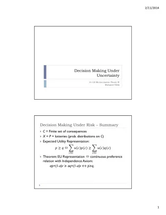
Decision Making Under Uncertainty Making Decisions Under - PDF document

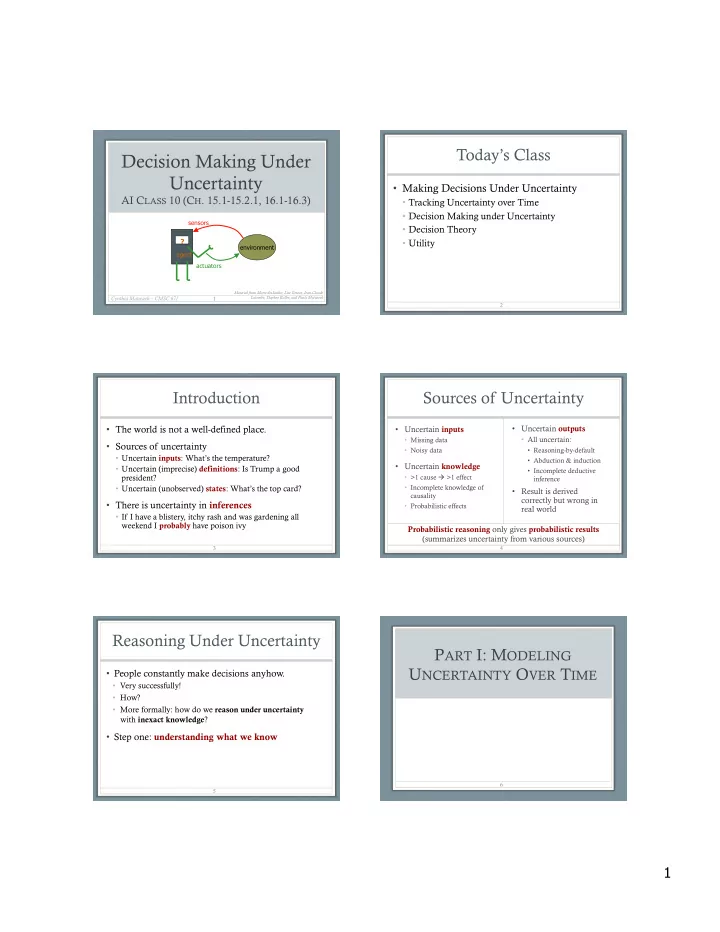
Today’s Class Decision Making Under Uncertainty • Making Decisions Under Uncertainty AI C LASS 10 (C H . 15.1-15.2.1, 16.1-16.3) • Tracking Uncertainty over Time • Decision Making under Uncertainty sensors • Decision Theory ? • Utility environment agent actuators Material from Marie desJardin, Lise Getoor, Jean-Claude Latombe, Daphne Koller, and Paula Matuszek Cynthia Matuszek – CMSC 671 1 2 Introduction Sources of Uncertainty • The world is not a well-defined place. • Uncertain inputs • Uncertain outputs • All uncertain: • Missing data • Sources of uncertainty • Noisy data • Reasoning-by-default • Uncertain inputs : What’s the temperature? • Abduction & induction • Uncertain knowledge • Uncertain (imprecise) definitions : Is Trump a good • Incomplete deductive president? • >1 cause à >1 effect inference • Incomplete knowledge of • Uncertain (unobserved) states : What’s the top card? • Result is derived causality correctly but wrong in • There is uncertainty in inferences • Probabilistic effects real world • If I have a blistery, itchy rash and was gardening all weekend I probably have poison ivy Probabilistic reasoning only gives probabilistic results (summarizes uncertainty from various sources) 4 3 Reasoning Under Uncertainty P ART I: M ODELING U NCERTAINTY O VER T IME • People constantly make decisions anyhow. • Very successfully! • How? • More formally: how do we reason under uncertainty with inexact knowledge ? • Step one: understanding what we know 6 5 1

States and Observations Temporal Probabilistic Agent • Agents don’t have a continuous view of world sensors • People don’t either! • We see things as a series of snapshots: ? environment • Observations , associated with time slices agent • t 1 , t 2 , t 3 , … actuators • Each snapshot contains all variables, observed or not • X t = (unobserved) state variables at time t; observation at t is E t t 1 , t 2 , t 3 , … • This is world state at time t 7 8 Uncertainty and Time Uncertainty and Time • The world changes • Basic idea: • Examples: diabetes management, traffic monitoring • Copy state and evidence variables for each time step • Model uncertainty in change over time • Tasks: track changes; predict changes • Incorporate new observations as they arrive • Basic idea: • X t = unobserved/unobservable state variables at time t: • For each time step, copy state and evidence variables BloodSugar t , StomachContents t • Model uncertainty in change over time (the Δ ) • E t = evidence variables at time t: • Incorporate new observations as they arrive MeasuredBloodSugar t , PulseRate t , FoodEaten t • Assuming discrete time steps 9 10 States (more formally) Observations (more formally) • Change is viewed as series of snapshots • Time slice (a set of random variables indexed by t ): • Time slices/timesteps 1. the set of unobservable state variables X t • Each describing the state of the world at a particular time 2. the set of observable evidence variables E t • So we also refer to these as states • An observation is a set of observed variable • Each time slice/timestep/state is represented as a instantiations at some timestep set of random variables indexed by t : • Observation at time t : E t = e t 1. the set of unobservable state variables X t • (for some values e t ) 2. the set of observable evidence variables E t • X a:b denotes the set of variables from X a to X b 11 12 2

Transition and Sensor Models Markov Assumption(s) • So how do we model change over time? • Markov Assumption : This can get • X t depends on some finite (usually fixed) number of previous X i ’s • Transition model exponentially • First-order Markov process : P( X t | X 0:t-1 ) = P( X t | X t-1 ) • Models how the world changes over time large… • Specifies a probability distribution… • k th order: depends on previous k time steps • Over state variables at time t P( X t | X 0:t-1 ) • Given values at previous times • Sensor model • Sensor Markov assumption : P( E t | X 0:t , E 0:t-1 ) = P( E t | X t ) • Models how evidence (sensor data) gets its values • E.g.: BloodSugar t à MeasuredBloodSugar t • Agent’s observations depend only on actual current state of the world 13 14 Stationary Process Complete Joint Distribution • Infinitely many possible values of t • Given: • Transition model: P( X t | X t-1 ) • Does each timestep need a distribution? • Sensor model: P( E t | X t ) • That is, do we need a distribution of what the world looks like at • Prior probability: P( X 0 ) t 3 , given t 2 AND a distribution for t 16 given t 15 AND … • Then we can specify a complete joint distribution • Assume stationary process : of a sequence of states: • Changes in the world state are governed by laws that do not themselves change over time t ∏ P ( X 0 , X 1 ,..., X t , E 1 ,..., E t ) = P ( X 0 ) P ( X i | X i − 1 ) P ( E i | X i ) • Transition model P( X t | X t-1 ) and sensor model P( E t | X t ) are time-invariant, i.e., they are the same for all t i = 1 • What’s the joint probability of instantiations? 15 16 Example Inference Tasks Weather has a 30% chance R t-1 P(R t | R t-1 ) • Filtering or monitoring: P( X t |e 1 ,…,e t ) : of changing and a 70% t 0.7 • Compute the current belief state, given all evidence to date chance of staying the same. f 0.3 • Prediction : P( X t+k |e 1 ,…,e t ) : Rain t-1 Rain t Rain t+1 • Compute the probability of a future state • Smoothing : P( X k |e 1 ,…, et ) : Umbrella t-1 Umbrella t Umbrella t+1 • Compute the probability of a past state (hindsight) • Most likely explanation : arg max x1,..xt P(x 1 ,…,x t |e 1 ,…,e t ) R t P(U t | R t ) • Given a sequence of observations, find the sequence of states that is t 0.9 f 0.2 most likely to have generated those observations Fully worked out HMM for rain: www2.isye.gatech.edu/~yxie77/isye6416_17/Lecture6.pdf 18 3

Examples Filtering • Filtering: What is the probability that it is raining today, • Maintain a current state estimate and update it given all of the umbrella observations up through today? • Instead of looking at all observed values in history • Prediction: What is the probability that it will rain the day • Also called state estimation after tomorrow, given all of the umbrella observations up through today? • Given result of filtering up to time t , agent must • Smoothing: What is the probability that it rained yesterday, compute result at t+ 1 from new evidence e t+1 : given all of the umbrella observations through today? P( X t+1 | e 1:t+1 ) = f ( e t+1 , P( X t | e 1:t )) • Most likely explanation: If the umbrella appeared the first three days but not on the fourth, what is the most likely … for some function f . weather sequence to produce these umbrella sightings? 19 20 Recursive Estimation Recursive Estimation 1. Project current state forward (t à t+1) • P( X t+1 | e 1:t+1 ) as a function of e t+1 and P( X t | e 1:t ): P ( X t + 1 | e 1: t + 1 ) = P ( X t + 1 | e 1: t , e t + 1 ) 2. Update state using new evidence e t+1 dividing up evidence = α P ( e t + 1 | X t + 1 , e 1: t ) P ( X t + 1 | e 1: t ) Bayes rule = α P ( e t + 1 | X t + 1 ) P ( X t + 1 | e 1: t ) sensor Markov assumption P( X t+1 | e 1:t+1 ) as function of e t+1 and P( X t | e 1:t ): • P( e t+1 | X 1:t+1 ) updates with new evidence (from sensor) P( X t +1 | e 1:t+1 ) = P( X t+1 | e 1:t , e t+1 ) • One-step prediction by conditioning on current state X: ∑ = α P ( e t + 1 | X t + 1 ) P ( X t + 1 | x t ) P ( x t | e 1: t ) x t 21 22 Group Exercise: Filtering Recursive Estimation ∑ P ( X t + 1 | e 1: t + 1 ) = α P ( e t + 1 | X t + 1 ) P ( X t + 1 | X t ) P ( X t | e 1: t ) • One-step prediction by conditioning on current state X: X t ∑ = α P ( e t + 1 | X t + 1 ) P ( X t + 1 | x t ) P ( x t | e 1: t ) R t-1 P(R t |R t-1 ) T 0.7 x t transition current F 0.3 model state Rain t-1 Rain t Rain t+1 • …which is what we wanted! • So, think of P( X t | e 1:t ) as a “message” f 1:t+1 • Carried forward along the time steps Umbrella t-1 Umbrella t Umbrella t+1 • Modified at every transition, updated at every new observation R t P(U t |R t ) • This leads to a recursive definition: What is the probability of rain on T 0.9 f 1:t+1 = α FORWARD ( f 1:t , e t+1 ) Day 2, given a uniform prior of rain F 0.2 on Day 0, U 1 = true, and U 2 = true? 23 24 4