Data Mining Graphical Models for Discrete Data Undirected Graphs - PowerPoint PPT Presentation
Data Mining Graphical Models for Discrete Data Undirected Graphs (Markov Random Fields) Ad Feelders Universiteit Utrecht Ad Feelders ( Universiteit Utrecht ) Data Mining 1 / 34 Overview of Coming Two Lectures Introduction Independence and
Data Mining Graphical Models for Discrete Data Undirected Graphs (Markov Random Fields) Ad Feelders Universiteit Utrecht Ad Feelders ( Universiteit Utrecht ) Data Mining 1 / 34
Overview of Coming Two Lectures Introduction Independence and Conditional Independence Graphical Representation of Conditional Independence Log-linear Models Hierarchical Graphical Decomposable Maximum Likelihood Estimation Model Testing Model Selection Ad Feelders ( Universiteit Utrecht ) Data Mining 2 / 34
Graphical Models for Discrete Data Task: model the associations (dependencies) between a collection of discrete variables. There is no designated target variable to be predicted: all variables are treated equal. This doesn’t mean these models can’t be used for prediction. They can! Ad Feelders ( Universiteit Utrecht ) Data Mining 3 / 34
Graphical Model for Right Heart Catheterization Data age ninsclas death race gender income cat1 swang1 is independent of meanbp1 ca death given cat1 swang1 Ad Feelders ( Universiteit Utrecht ) Data Mining 4 / 34
An example Consider the following table of counts on X and Y : n ( x , y ) y x q r s n ( x ) a 2 5 3 10 b 10 20 10 40 c 8 35 7 50 n ( y ) 20 60 20 100 Suppose we want to estimate the joint distribution of X and Y . Ad Feelders ( Universiteit Utrecht ) Data Mining 5 / 34
The Saturated Model Saturated (unconstrained) model P ( x , y ) = n ( x , y ) ˆ n requires the estimation of 8 probabilities. n ( x , y ) = n ˆ The fitted counts ˆ P ( x , y ) are the same as the observed counts. ˆ P ( x , y ) y n ( x , y ) ˆ y ˆ x q r s n ( x ) ˆ x q r s P ( x ) a 2 5 3 10 a 0.02 0.05 0.03 0.1 b 10 20 10 40 b 0.10 0.20 0.10 0.4 c 8 35 7 50 c 0.08 0.35 0.07 0.5 n ( y ) ˆ 20 60 20 100 ˆ P ( y ) 0.2 0.6 0.2 1 Ad Feelders ( Universiteit Utrecht ) Data Mining 6 / 34
The Saturated Model and the Curse of Dimensionality The saturated model estimates cell probabilities by dividing the cell count by the total number of observations. It makes no simplifying assumptions. This approach doesn’t scale very well! Suppose we have k categorical variables with m possible values each. To estimate the probability of each possible combination of values would require the estimation of m k probabilities. For k = 10 and m = 5, this is 5 10 ≈ 10 million probabilities This is a manifestation of the curse of dimensionality : we have fewer data points than probabilities to estimate. Estimates will become unreliable. Ad Feelders ( Universiteit Utrecht ) Data Mining 7 / 34
How to avoid this curse Make independence assumptions to obtain a simpler model that still gives a good fit. Independence Model P ( y ) = n ( x ) n ( y ) = n ( x ) n ( y ) P ( x , y ) = ˆ ˆ P ( x ) ˆ n 2 n n requires the estimation of just 4 probabilities instead of 8. Ad Feelders ( Universiteit Utrecht ) Data Mining 8 / 34
Fit of independence model The fitted counts of the independence model are given by P ( x , y ) = n n ( x ) n ( y ) = n ( x ) n ( y ) n ( x , y ) = n ˆ ˆ n 2 n For example n ( x = b , y = s ) = n ( x = b ) n ( y = s ) = 40 × 20 ˆ = 8 n 100 Compare the fitted counts (left) with the observed counts (right): n ( x , y ) ˆ y n ( x , y ) y x q r s n ( x ) ˆ x q r s n ( x ) a 2 6 2 10 a 2 5 3 10 b 8 24 8 40 b 10 20 10 40 c 10 30 10 50 c 8 35 7 50 n ( y ) ˆ 20 60 20 100 n ( y ) 20 60 20 100 Ad Feelders ( Universiteit Utrecht ) Data Mining 9 / 34
Fit of independence model The fitted counts of the independence model are quite close to the observed counts. We could conclude that the independence model gives a satisfactory fit of the data. Use a statistical test to make this more precise (discussed later). Ad Feelders ( Universiteit Utrecht ) Data Mining 10 / 34
Independence Model The saturated model requires the estimation of m k − 1 probabilities. The mutual independence model requires just k ( m − 1) probability estimates. Mutual independence model is usually not appropriate (all variables are independent of one another). Interesting models are somewhere in between saturated and mutual independence: this requires the notion of conditional independence. Ad Feelders ( Universiteit Utrecht ) Data Mining 11 / 34
Rules of Probability 1 Sum Rule: � P ( X ) = P ( X , Y ) Y 2 Product Rule: P ( X , Y ) = P ( X ) P ( Y | X ) 3 If X and Y are independent, then P ( X , Y ) = P ( X ) P ( Y ) Ad Feelders ( Universiteit Utrecht ) Data Mining 12 / 34
Independence of (sets of) random variables Let X and Y be (sets of) random variables. X and Y are independent if and only if: P ( x , y ) = P ( x ) P ( y ) for all values ( x , y ) . Equivalently: P ( x | y ) = P ( x ) , and P ( y | x ) = P ( y ) Y doesn’t provide any information about X (and vice versa) We also write X ⊥ ⊥ Y . For example: gender is independent of eye color. Ad Feelders ( Universiteit Utrecht ) Data Mining 13 / 34
Factorisation criterion for independence We can relax our burden of proof a little bit: X and Y are independent iff there are functions g ( x ) and h ( y ) (not necessarily the marginal distributions of X and Y ) such that P ( x , y ) = g ( x ) h ( y ) In logarithmic form this becomes (since log ab = log a + log b ): log P ( x , y ) = g ∗ ( x ) + h ∗ ( y ) , where g ∗ ( x ) = log g ( x ). Ad Feelders ( Universiteit Utrecht ) Data Mining 14 / 34
Factorisation criterion for independence: proof Suppose that for all x and y : P ( x , y ) = g ( x ) h ( y ) Then � � � P ( x ) = P ( x , y ) = g ( x ) h ( y ) = g ( x ) h ( y ) = c 1 g ( x ) y y y So g ( x ) is proportional to P ( x ). Likewise, h ( y ) is proportional to P ( y ). Therefore P ( x , y ) = g ( x ) h ( y ) = 1 P ( x ) 1 P ( y ) = c 3 P ( x ) P ( y ) c 1 c 2 Summing over both x and y establishes that c 3 = 1, so X and Y are independent. Ad Feelders ( Universiteit Utrecht ) Data Mining 15 / 34
Conditional Independence X and Y are conditionally independent given Z iff P ( x , y | z ) = P ( x | z ) P ( y | z ) (1) for all values ( x , y ) and for all values z for which P ( z ) > 0. Equivalently: P ( x | y , z ) = P ( x | z ) If I already know the value of Z, then Y doesn’t provide any additional information about X. We also write X ⊥ ⊥ Y | Z . For example: ice cream sales is independent of mortality among the elderly given the weather. Ad Feelders ( Universiteit Utrecht ) Data Mining 16 / 34
The Causal Picture Temp. + + + Sales Mortality P(Mortality = hi | Sales = hi) � = P(Mortality = hi) P(Mortality = hi | Temp. = hi, Sales = hi) = P(Mortality = hi | Temp. = hi) Ad Feelders ( Universiteit Utrecht ) Data Mining 17 / 34
Factorisation Criterion for Conditional Independence An equivalent formulation is (multiply equation (1) by P ( z )): P ( x , y , z ) = P ( x , z ) P ( y , z ) P ( z ) Factorisation criterion: X ⊥ ⊥ Y | Z iff there exist functions g and h such that P ( x , y , z ) = g ( x , z ) h ( y , z ) or alternatively log P ( x , y , z ) = g ∗ ( x , z ) + h ∗ ( y , z ) for all ( x , y ) and for all z for which P ( z ) > 0. Ad Feelders ( Universiteit Utrecht ) Data Mining 18 / 34
Conditional Independence Graph Random Vector X = ( X 1 , X 2 , . . . , X k ) with probability distribution P ( X ). Graph G = ( K , E ), with K = { 1 , 2 , . . . , k } . The conditional independence graph of X is the undirected graph G = ( K , E ) where { i , j } is not in the edge set E if and only if: X i ⊥ ⊥ X j | rest Ad Feelders ( Universiteit Utrecht ) Data Mining 19 / 34
Conditional Independence Graph: Example X = ( X 1 , X 2 , X 3 , X 4 ) , 0 < x i < 1 with probability density P ( x ) = e c + x 1 + x 1 x 2 + x 2 x 3 x 4 Now log P ( x ) = c + x 1 + x 1 x 2 + x 2 x 3 x 4 Application of the factorisation criterion gives X 1 ⊥ ⊥ X 4 | ( X 2 , X 3 ) and X 1 ⊥ ⊥ X 3 | ( X 2 , X 4 ) , For example log P ( x ) = c + x 1 + x 1 x 2 + x 2 x 3 x 4 � �� � � �� � g ( x 1 , x 2 , x 3 ) h ( x 2 , x 3 , x 4 ) Hence, the conditional independence graph is: 1 2 4 3 Ad Feelders ( Universiteit Utrecht ) Data Mining 20 / 34
Separation and Conditional Independence Consider the following conditional independence graph: 1 2 3 7 4 5 6 X 1 ⊥ ⊥ X 3 | ( X 2 , X 4 , X 5 , X 6 , X 7 ) Ad Feelders ( Universiteit Utrecht ) Data Mining 21 / 34
{ 2 , 5 } separates 1 from 3 Consider the following conditional independence graph: 1 2 3 7 4 5 6 X 1 ⊥ ⊥ X 3 | ( X 2 , X 4 , X 5 , X 6 , X 7 ) { 2 , 5 } separates 1 from 3 ⇒ X 1 ⊥ ⊥ X 3 | ( X 2 , X 5 ) Ad Feelders ( Universiteit Utrecht ) Data Mining 22 / 34
Separation and Conditional Independence Notation: X a = ( X i : i ∈ a ) where a is a subset of { 1 , 2 , . . . , k } . For example, if a = { 1 , 3 , 6 } then X a = ( X 1 , X 3 , X 6 ). The set a separates node i from node j iff every path from node i to node j contains one or more nodes in a (every path “goes through” a ). a separates b from c ( a , b , c disjoint): For every i ∈ b and j ∈ c : a separates i from j Ad Feelders ( Universiteit Utrecht ) Data Mining 23 / 34
Recommend
More recommend
Explore More Topics
Stay informed with curated content and fresh updates.

