CSCE 970 Lecture 4: Introduction to Bayesian Networks E.g. each - PDF document

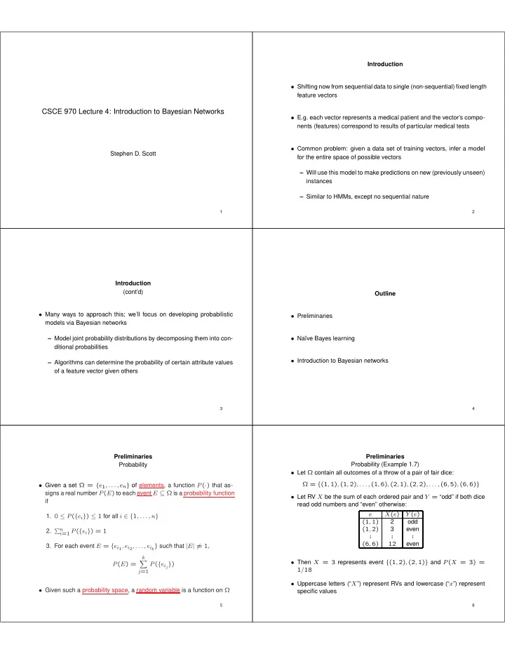
Introduction • Shifting now from sequential data to single (non-sequential) fixed length feature vectors CSCE 970 Lecture 4: Introduction to Bayesian Networks • E.g. each vector represents a medical patient and the vector’s compo- nents (features) correspond to results of particular medical tests • Common problem: given a data set of training vectors, infer a model Stephen D. Scott for the entire space of possible vectors – Will use this model to make predictions on new (previously unseen) instances – Similar to HMMs, except no sequential nature 1 2 Introduction (cont’d) Outline • Many ways to approach this; we’ll focus on developing probabilistic • Preliminaries models via Bayesian networks – Model joint probability distributions by decomposing them into con- • Na¨ ıve Bayes learning ditional probabilities • Introduction to Bayesian networks – Algorithms can determine the probability of certain attribute values of a feature vector given others 3 4 Preliminaries Preliminaries Probability Probability (Example 1.7) • Let Ω contain all outcomes of a throw of a pair of fair dice: Ω = { (1 , 1) , (1 , 2) , . . . , (1 , 6) , (2 , 1) , (2 , 2) , . . . , (6 , 5) , (6 , 6) } • Given a set Ω = { e 1 , . . . , e n } of elements, a function P ( · ) that as- signs a real number P ( E ) to each event E ⊆ Ω is a probability function • Let RV X be the sum of each ordered pair and Y = “odd” if both dice if read odd numbers and “even” otherwise: e X ( e ) Y ( e ) 1. 0 ≤ P ( { e i } ) ≤ 1 for all i ∈ { 1 , . . . , n } (1 , 1) 2 odd (1 , 2) 3 even 2. � n i =1 P ( { e i } ) = 1 . . . . . . . . . (6 , 6) 12 even 3. For each event E = { e i 1 , e i 2 , . . . , e i k } such that | E | � = 1 , k • Then X = 3 represents event { (1 , 2) , (2 , 1) } and P ( X = 3) = P ( E ) = � P ( { e i j } ) 1 / 18 j =1 • Uppercase letters (“ X ”) represent RVs and lowercase (“ x ”) represent • Given such a probability space, a random variable is a function on Ω specific values 5 6

Preliminaries Marginal Probability Preliminaries Joint Distributions • If we have a handle on a joint distribution, we can sum across values of an RV to get the marginal probability distribution of another RV • In previous example, X ranged over the integers 2–12 and Y ranged over { odd,even } • For two RVs X and Y , � P ( X = x ) = P ( X = x, Y = y ) – Each value in each range had its own probability y • E.g. • If we consider joint events (one from X ’s range, one from Y ’s) we get P ( X = 4) = � P ( X = 4 , Y = y ) a joint probability distribution P ( x, y ) = P ( X = x, Y = y ) y = P ( X = 4 , Y = odd ) + P ( X = 4 , Y = even ) = 1 / 18 + 1 / 36 = 1 / 12 • E.g. x = 4 and y = odd represents the event { (1 , 3) , (3 , 1) } and P ( x, y ) = 1 / 18 • Also see Example 1.15 7 8 Preliminaries Preliminaries Conditional Probability Bayes’ Theorem • Let E and F be events with P ( F ) > 0 • An identity for conditional probabilities • The conditional probability of E given F is • Given two events E and F with P ( E ) , P ( F ) > 0 P ( E | F ) = P ( E ∩ F ) P ( E | F ) = P ( F | E ) P ( E ) P ( F ) P ( F ) (Way to remember: the event named after the line goes in the denom- inator) • E.g. if x = 6 and y = even then P ( X = x ) = • E.g. When x = 6 and y = even, P ( X = x, Y = y ) = P ( x | y ) = P ( y | x ) P ( x ) = (2 / 5)(5 / 36) = 2 / 27 P ( y ) 27 / 36 P ( X = x | Y = y ) = 9 10 Preliminaries Independence of Events Preliminaries Conditional Independence of Events • Two events E and F are independent if one of the following holds: 1. P ( E | F ) = P ( E ) and P ( E ) , P ( F ) � = 0 • Can also have independence conditioned on other variables (can switch roles of E and F for same result) 2. P ( E ) = 0 or P ( F ) = 0 • Events E and F are conditionally independent given G if P ( G ) > 0 and one of the following holds • E and F are independent iff P ( E ∩ F ) = P ( E ) P ( F ) 1. P ( E | F ∩ G ) = P ( E | G ) and P ( E | G ) , P ( F | G ) > 0 • E.g. is the event X = 6 independent of Y = even? 2. P ( E | G ) = 0 or P ( F | G ) = 0 • Is the event X = 10 ∪ X = 12 independent of Y = odd? 11 12

Preliminaries Preliminaries Conditional Independence of Events Independence of Random Variables Example • Given probability space (Ω , P ) , two RVs A and B are independent • Define third RV Z , defined as the product of the two dice results (written I P ( A, B ) ) if, for all values a of A and b of B , the events A = a P ( X = 5 | Y = even ) = 4 / 36 and B = b are independent 27 / 36 = 4 / 27 � = 4 / 36 = P ( X = 5) P ( X = 5 | Y = even ∩ Z = 4) = 2 / 36 • I.e. for all values a and b , either P ( a ) = 0 or P ( b ) = 0 or 3 / 36 = 2 / 3 = P ( X = 5 | Z = 4) P ( a | b ) = P ( a ) • Thus the event X = 5 is not independent of Y = even, but is condi- • Generalizes to sets of RVs tionally independent of it given Z = 4 13 14 Preliminaries Independence of Random Variables Preliminaries Example 1.16 Conditional Independence of Random Variables Ω = set of all cards in a deck, P uniform Variable Values Outcomes • Given probability space (Ω , P ) , two RVs A and B are R { r 1 , r 2 } royal/nonroyal cards conditionally independent given C (written I P ( A, B | C ) ) if, for all T { t 1 , t 2 } tens & jacks/not t & j S { s 1 , s 2 } spades/nonspades values a of A , b of B , and c of C , the events A = a and B = b are conditionally independent given event C = c s r t P ( r, t | s ) P ( r, t ) s 1 r 1 t 1 1 / 13 4 / 52 = 1 / 13 s 1 r 1 t 2 2 / 13 8 / 52 = 2 / 13 • I.e. for all values a and b and c , either P ( a | c ) = 0 or P ( b | c ) = 0 or s 1 r 2 t 1 1 / 13 4 / 52 = 1 / 13 s 1 r 2 t 2 9 / 13 36 / 52 = 9 / 13 P ( a | b, c ) = P ( a | c ) s 2 r 1 t 1 3 / 39 = 1 / 13 4 / 52 = 1 / 13 s 2 r 1 t 2 6 / 39 = 2 / 13 8 / 52 = 2 / 13 s 2 r 2 t 1 3 / 39 = 1 / 13 4 / 52 = 1 / 13 • Generalizes to sets of RVs s 2 r 2 t 2 27 / 39 = 9 / 13 36 / 52 = 9 / 13 Thus P ( r, t | s ) = P ( r, t ) ⇒ I P ( { R, T } , { S } ) 15 16 Preliminaries Basic Formulas for Probabilities Conditional Independence of Random Variables, Example 1.17 • Product Rule: probability P ( A ∩ B ) of conjunction of events A and B: P ( A ∩ B ) = P ( A | B ) P ( B ) = P ( B | A ) P ( A ) • Sum Rule: probability of a disjunction of two events A and B: P ( A ∪ B ) = P ( A ) + P ( B ) − P ( A ∩ B ) P is uniform c s v P ( v | s, c ) P ( v | c ) • Theorem of total probability: if events A 1 , . . . , A n are mutually exclu- c 1 s 1 v 1 1 / 3 3 / 9 = 1 / 3 sive with � n i =1 P ( A i ) = 1 , then c 1 s 1 v 2 2 / 3 6 / 9 = 2 / 3 Var Values Outcomes n c 1 s 2 v 1 1 / 3 3 / 9 = 1 / 3 � P ( B ) = P ( B | A i ) P ( A i ) V { v 1 , v 2 } obj with “1”/“2” c 1 s 2 v 2 2 / 3 6 / 9 = 2 / 3 i =1 S { s 1 , s 2 } square/round c 2 s 1 v 1 1 / 2 2 / 4 = 1 / 2 C { c 1 , c 2 } black/white c 2 s 1 v 2 1 / 2 2 / 4 = 1 / 2 • If X takes on real values, then its expected value is c 2 s 2 v 1 1 / 2 2 / 4 = 1 / 2 � c 2 s 2 v 2 1 / 2 2 / 4 = 1 / 2 E ( X ) = xP ( x ) x Thus P ( v | s, c ) = P ( v | c ) ⇒ I P ( { V } , { S } | { C } ) 17 18