CSCE 970 Lecture 2: most probable class Bayesian-Based Classifiers - PDF document

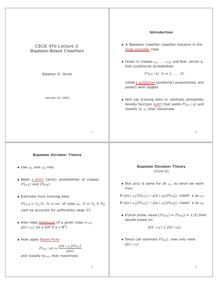
Introduction • A Bayesian classifier classifies instance in the CSCE 970 Lecture 2: most probable class Bayesian-Based Classifiers • Given M classes ω 1 , . . . , ω M and feat. vector x , find conditional probabilities P ( ω i | x ) ∀ i = 1 , . . . , M, Stephen D. Scott called a posteriori (posterior) probabilities, and predict with largest January 10, 2001 • Will use training data to estimate probability density function (pdf) that yields P ( ω i | x ) and classify to ω i that maximizes 2 1 Bayesian Decision Theory Bayesian Decision Theory • Use ω 1 and ω 2 only (Cont’d) • Need a priori (prior) probabilities of classes: • But p ( x ) is same for all ω i , so since we want P ( ω 1 ) and P ( ω 2 ) max: If p ( x | ω 1 ) P ( ω 1 ) > p ( x | ω 2 ) P ( ω 2 ), classif. x as ω 1 • Estimate from training data: If p ( x | ω 1 ) P ( ω 1 ) < p ( x | ω 2 ) P ( ω 2 ), classif. x as ω 2 P ( ω i ) ≈ N i /N, N i = no. of class ω i , N = N 1 + N 2 (will be accurate for sufficiently large N ) • If prior probs. equal ( P ( ω 1 ) = P ( ω 2 ) = 1 / 2) then decide based on: • Also need likelihood of x given class = ω i : p ( x | ω i ) (is a pdf if x ∈ ℜ ℓ ) p ( x | ω 1 ) ≷ p ( x | ω 2 ) • Now apply Bayes Rule: • Since can estimate P ( ω i ), now only need p ( x | ω i ) P ( ω i | x ) = p ( x | ω i ) P ( ω i ) p ( x ) and classify to ω i that maximizes 3 4

Bayesian Decision Theory Bayesian Decision Theory Example Probability of Error • In general, error is P e = P ( x ∈ R 2 , ω 1 ) + P ( x ∈ R 1 , ω 2 ) = P ( x ∈ R 2 | ω 1 ) P ( ω 1 ) + P ( x ∈ R 1 | ω 2 ) P ( ω 2 ) � � = P ( ω 1 ) p ( x | ω 1 ) d x + P ( ω 2 ) p ( x | ω 2 ) d x R 2 R 1 � � = P ( ω 1 | x ) p ( x ) d x + P ( ω 2 | x ) p ( x ) d x R 2 R 1 • Since R 1 and R 2 cover entire space, � � P ( ω 1 | x ) p ( x ) d x + P ( ω 1 | x ) p ( x ) d x = P ( ω 1 ) R 1 R 2 • Thus • ℓ = 1 feature, P ( ω 1 ) = P ( ω 2 ), so predict at � dotted line P e = P ( ω 1 ) − ( P ( ω 1 | x ) − P ( ω 2 | x )) p ( x ) d x , R 1 which is minimized if • Total error probability = shaded area: � � x ∈ ℜ ℓ : P ( ω 1 | x ) > P ( ω 2 | x ) R 1 = , � x 0 � + ∞ P e = −∞ p ( x | ω 2 ) dx + p ( x | ω 1 ) dx which is what the Bayesian classifier does! x 0 5 6 Bayesian Decision Theory Minimizing Risk • What if different errors have different penal- ties, e.g. cancer diagnosis? – False negative worse than false positive Bayesian Decision Theory • Define λ ki as loss (penalty, risk) if we pre- ℓ > 2 dict ω i when correct answer is ω k (forms L = loss matrix) • If number of classes ℓ > 2, then classify according to • Can minimize average loss: prob. of error ki argmax P ( ω i | x ) M M � �� � � ω i � � r = P ( ω k ) λ ki p ( x | ω k ) d x R i k =1 i =1   M M � • Proof of optimality still holds � �  d x = λ ki p ( x | ω k ) P ( ω k )  R i i =1 k =1 by minimizing each integral:  M   x ∈ ℜ ℓ : � R i = λ ki p ( x | ω k ) P ( ω k ) k =1  M  � < λ kj p ( x | ω k ) P ( ω k ) ∀ j � = i  k =1 7 8

Discriminant Functions • Rather than using probabilities (or risk func- tions) directly, sometimes easier to work with Bayesian Decision Theory a function of them, e.g. Minimizing Risk Example g i ( x ) = f ( P ( ω i | x )) f ( · ) is monotonically increasing function, g i ( x ) � � 0 λ 12 is called discriminant function • Let ℓ = 2, P ( ω 1 ) = P ( ω 2 ) = 1 / 2, L = , λ 21 0 and λ 21 > λ 12 � � x ∈ ℜ ℓ : g i ( x ) > g j ( x ) ∀ j � = i • Then R i = • Then � � x ∈ ℜ 2 : λ 21 p ( x | ω 2 ) > λ 12 p ( x | ω 1 ) • Common choice of f ( · ) is natural logarithm R 2 = (multiplications become sums) � � x ∈ ℜ 2 : p ( x | ω 2 ) > p ( x | ω 1 ) λ 12 = , λ 21 • Still requires good estimate of pdf which slides threshold left of x 0 on slide 5 since λ 12 /λ 21 < 1 – Will look at a tractable case next – In general, cannot necessarily easily esti- mate pdf, so use other cost functions (Chap- ters 3 & 4) 9 10 Normal Distributions Normal Distributions Minimum Distance Classifiers • Assume the pdf of likelihood functions follow a • If P ( ω i )’s equal and Σ i ’s equal, can use: normal (Gaussian) distribution for 1 ≤ i ≤ M : g i ( x ) = − 1 2( x − µ i ) T Σ − 1 ( x − µ i ) � � 1 − 1 2( x − µ i ) T Σ − 1 p ( x | ω i ) = (2 π ) ℓ/ 2 | Σ i | 1 / 2 exp ( x − µ i ) i • If features statistically independent with same · µ i = E [ x ] = mean value of ω i class variance, then Σ = σ 2 I and can instead use · | Σ i | = determinant of Σ i , ω i ’s covariance matrix: ℓ g i ( x ) = − 1 � ( x j − µ ij ) 2 � ( x − µ i )( x − µ i ) T � 2 Σ i = E j =1 – Assume we know µ i and Σ i ∀ i • Finding ω i maximizing this implies finding µ i that minimizes Euclidian distance to x • Using the following discriminant function: – Constant distance = circle centered at µ i g i ( x ) = ln( p ( x | ω i ) P ( ω i )) we get: • If Σ not diagonal, then maximizing g i ( x ) is same as minimizing Mahalanobis distance: g i ( x ) = − 1 2( x − µ i ) T Σ − 1 ( x − µ i ) + ln( P ( ω i )) i � ( x − µ i ) T Σ − 1 ( x − µ i ) − ℓ/ 2 ln(2 π ) − (1 / 2) ln | Σ i | – Constant distance = ellipse centered at µ i 11 12

Estimating Unknown pdf’s Estimating Unknown pdf’s ML Param Est (cont’d) Maximum Likelihood Parameter Estimation • Assuming statistical indep. of x ki ’s, Σ − 1 = 0 ij for i � = j , so • If we know cov. matrix but not mean for a � �  � 2 Σ − 1  � class ω , can parameterize ω ’s pdf on mean µ : ∂   − 1 � N � ℓ ∂L x kj − µ j k =1 j =1 jj ∂µ 1 2 ∂µ 1   ∂L . . � �     1 − 1 . . ∂ µ = .  = . 2( x k − µ ) T Σ − 1 ( x k − µ )     p ( x k ; µ ) = (2 π ) ℓ/ 2 | Σ | 1 / 2 exp    � � � 2 Σ − 1 ∂L �   ∂ − 1 � N � ℓ x kj − µ j ∂µ ℓ ∂µ ℓ k =1 j =1 jj 2 and use data x 1 , . . . , x N from ω to estimate µ N � Σ − 1 ( x k − µ ) = 0 , = k =1 • The maximum likelihood (ML) method esti- mates µ such that the following likelihood func- yielding tion is maximized: N µ ML = 1 � N ˆ x k � N p ( X ; µ ) = p ( x 1 , . . . , x N ; µ ) = p ( x k ; µ ) k =1 k =1 • Solve above for each class independently • Taking logarithm and setting gradient = 0 :   • Can generalize technique for other N − 1 ∂  − N � � � (2 π ) ℓ | Σ | ( x k − µ ) T Σ − 1 ( x k − µ ) 2 ln = 0  distributions and parameters ∂ µ 2 k =1 � �� � L • Has many nice properties (p. 30) as N → ∞ 14 13 Estimating Unknown pdf’s Estimating Unknown pdf’s Maximum A Posteriori Parameter Estimation (Nonparametric Approach) Parzen Windows • If µ is norm. distrib., Σ = σ 2 µ I , mean = µ 0 : � � − ( µ − µ 0 ) T ( µ − µ 0 ) • Historgram-based technique to approximate pdf: 1 p ( µ ) = exp Partition space into “bins” and count number (2 π ) ℓ/ 2 σ ℓ 2 σ 2 µ µ of training vectors per bin • Maximizing p ( µ | X ) is same as maximizing p(x) N � p ( µ ) p ( X | µ ) = p ( x k | µ ) p ( µ ) k =1 • Again, take log and set gradient = 0: (Σ = σ 2 I ) N σ 2 ( x k − µ ) − 1 1 � ( µ − µ 0 ) = 0 x σ 2 µ k =1 so  1 if | x j | ≤ 1 / 2 µ MAP = µ 0 + ( σ 2 µ /σ 2 ) � N  k =1 x k • Let φ ( x ) = ˆ 0 otherwise 1 + ( σ 2 µ /σ 2 ) N  • Now approximate pdf p ( x ) with • µ MAP ≈ µ ML if p ( µ ) almost uniform or N → ∞  � N � x i − x p ( x ) = 1  1 � ˆ φ  • Again, can generalize technique h ℓ N h i =1 15 16

Estimating Unknown pdf’s Estimating Unknown pdf’s Parzen Windows Parzen Windows (cont’d) Numeric Example  � N � x i − x p ( x ) = 1  1 � ˆ φ  h ℓ N h i =1 • I.e. given x , to compute ˆ p ( x ): – Count number of training vectors in size- h (per side) hypercube H centered at x – Divide by N to est. probability of getting a point in H – Divide by volume of H • Problem: Approximating continuous function p ( x ) with discontinuous ˆ p ( x ) • Solution: Substitute a smooth function for � 1 / (2 π ) ℓ/ 2 � � � − x T x / 2 φ ( · ), e.g. φ ( x ) = exp 18 17 k -Nearest Neighbor Techniques • Classify unlabeled feature vector x according to a majority vote of its k nearest neighbors k = 3 Euclidean distance = Class A = Class B = unclassified (predict B) • As N → ∞ , – 1-NN error is at most twice Bayes opt. ( P B ) √ – k -NN error is ≤ P B + 1 / ke • Can also weight votes by relative distance • Complexity issues: Research into more effi- cient algorithms, approximation algorithms 19