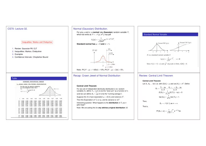

CS70: Lecture 32. Normal (Gaussian) Distribution. For any µ and σ , a normal (aka Gaussian ) random variable Y , which we write as Y = N ( µ , σ 2 ) , has pdf 1 2 πσ 2 e − ( y − µ ) 2 / 2 σ 2 . f Y ( y ) = √ Inequalities: Markov and Chebyshev Standard normal has µ = 0 and σ = 1 . 1. Review: Gaussian RV, CLT 2. Inequalities: Markov, Chebyshev 3. Examples 4. Confidence Intervals: Cheybshev Bound Note: Pr [ | Y − µ | > 1 . 65 σ ] = 10 %; Pr [ | Y − µ | > 2 σ ] = 5 % . Recap: Crown Jewel of Normal Distribution Review: Central Limit Theorem Central Limit Theorem Let X 1 , X 2 ,... be i.i.d. with E [ X 1 ] = µ and var ( X 1 ) = σ 2 . Define Central Limit Theorem S n := T n − n µ = X 1 + ··· + X n − n µ σ √ n σ √ n . For any set of independent identically distributed (i.i.d.) random variables X i , define T n = ∑ X i to be the “total sum” as a function of n . 1 σ √ n ( E ( T n ) − n µ ) = 0 E ( S n ) = (and we can define A n = 1 n ∑ X i to be the “running average.”) 1 Suppose the X i ’s have expectation µ = E ( X i ) and variance σ 2 . Var ( S n ) = σ 2 nVar ( T n ) = 1 . Then the Expectation of T n is n µ , and its variance is n σ 2 . Then, Interesting question: What happens to the distribution of T n as n S n → N ( 0 , 1 ) , as n → ∞ . gets large? That is, Note: We are asking this for any arbitrary original distribution X i ! � α 1 − ∞ e − x 2 / 2 dx . Pr [ S n ≤ α ] → √ 2 π
n n µ µ a n Inequalities: An Overview Andrey Markov Chebyshev Distribution Markov Andrey Markov is best known for his work on stochastic processes. A primary subject of his p n p n p n research later became known as Markov chains and Markov processes. Pafnuty Chebyshev was one of his teachers. � � Markov was an atheist. In 1912 he protested p n Leo Tolstoy’s excommunication from the Russian Orthodox Church by requesting his own excommunication. The Church complied P r [ X > a ] P r [ | X − µ | > � ] with his request.
Markov’s inequality (General Form) A picture The inequality is named after Andrey Markov, although it appeared earlier in the work of Pafnuty Chebyshev. It should be (and is sometimes) called Chebyshev’s first inequality. Theorem Markov’s Inequality Assume f : ℜ → [ 0 , ∞ ) is nondecreasing. Then, Pr [ X ≥ a ] ≤ E [ f ( X )] , for all a such that f ( a ) > 0 . f ( a ) Proof: Observe that 1 { X ≥ a } ≤ f ( X ) f ( a ) . Indeed, if X < a , the inequality reads 0 ≤ f ( X ) / f ( a ) , which holds since f ( · ) ≥ 0. Also, if X ≥ a , it reads 1 ≤ f ( X ) / f ( a ) , which holds since f ( · ) is nondecreasing. Taking the expectation yields the inequality, because expectation is monotone. Chebyshev’s Inequality This is Pafnuty’s inequality: Theorem: Pr [ | X − E [ X ] | > a ] ≤ var [ X ] , for all a > 0 . a 2 Proof: Let Y = | X − E [ X ] | and f ( y ) = y 2 . Then, Pr [ Y ≥ a ] ≤ E [ f ( Y )] = var [ X ] . a 2 f ( a ) This result confirms that the variance measures the “deviations from the mean.”
Fraction of H ’s Here is a classical application of Chebyshev’s inequality. How likely is it that the fraction of H ’s differs from 50 % ? Let X m = 1 if the m -th flip of a fair coin is H and X m = 0 otherwise. Define M n = X 1 + ··· + X n , for n ≥ 1 . n We want to estimate Pr [ | M n − 0 . 5 | ≥ 0 . 1 ] = Pr [ M n ≤ 0 . 4 or M n ≥ 0 . 6 ] . By Chebyshev, Pr [ | M n − 0 . 5 | ≥ 0 . 1 ] ≤ var [ M n ] ( 0 . 1 ) 2 = 100 var [ M n ] . Now, var [ M n ] = 1 n 2 ( var [ X 1 ]+ ··· + var [ X n ]) = 1 n var [ X 1 ] ≤ 1 4 n . Var ( X i ) = p ( 1 − lp ) ≤ ( . 5 )( . 5 ) = 1 4 Fraction of H ’s Summary M n = X 1 + ··· + X n , for n ≥ 1 . n Pr [ | M n − 0 . 5 | ≥ 0 . 1 ] ≤ 25 n . Inequalities: Markov and Chebyshev For n = 1 , 000, we find that this probability is less than 2 . 5 % . As n → ∞ , this probability goes to zero. 1. Inequalities: Markov and Chebyshev Tail Bounds In fact, for any ε > 0, as n → ∞ , the probability that the fraction 2. Confidence Intervals: Chebyshev Bounds of H s is within ε > 0 of 50 % approaches 1: Pr [ | M n − 0 . 5 | ≤ ε ] → 1 . This is an example of the (Weak) Law of Large Numbers. We will address WLLN next time.
Recommend
More recommend