Lecture 3: The Normal Distribution and Statistical Inference Ani - PowerPoint PPT Presentation
Lecture 3: The Normal Distribution and Statistical Inference Ani Manichaikul amanicha@jhsph.edu 19 April 2007 1 / 62 A Review and Some Connections The Normal Distribution The Central Limit Theorem Estimates of means and proportions: uses
Lecture 3: The Normal Distribution and Statistical Inference Ani Manichaikul amanicha@jhsph.edu 19 April 2007 1 / 62
A Review and Some Connections The Normal Distribution The Central Limit Theorem Estimates of means and proportions: uses and properties Confidence intervals and Hypothesis tests 2 / 62
The Normal Distribution Probability distribution for continuous data Under certain conditions , can be used to approximate binomial probabilities np > 5 n(1-p) > 5 Characterized by a symmetric bell-shaped curve (Gaussian curve) Symmetric about its mean µ 3 / 62
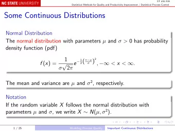
Normal Distribution Takes on values between −∞ and + ∞ Mean = Median = Mode Area under curve equals 1 Parameters µ = mean σ = standard deviation 4 / 62
Normal Distribution Normal Density µ −∞ + ∞ Notation for Normal random variable: X ∼ N ( µ, σ 2 ) 5 / 62
Formula: Normal Distribution The normal probability distribution is given by: 1 · e − ( x − µ ) 2 / 2 σ 2 , −∞ < x < + ∞ f ( x ) = √ 2 πσ π ≈ 3 . 14 and e ≈ 2 . 72 are mathematical constants µ, σ are mean and SD parameters of the distribution 6 / 62
Standard Normal The standard normal distribution has parameters µ = 0 and σ = 1 Its density function is written as: 1 · e − x 2 / 2 , −∞ < x < + ∞ f ( x ) = √ 2 π We typically use the letter Z to denote a standard normal random variable ( Z ∼ N (0 , 1)) If X ∼ N ( µ, σ ), then X − µ ∼ N (0 , 1) σ 7 / 62
68-95-99.7 Rule I 68% of density is within one standard deviation of the mean 8 / 62
68-95-99.7 Rule II 95% of density is within two standard deviations of the mean 9 / 62
68-95-99.7 Rule III 99.7% of density is within three standard deviations of the mean 10 / 62
Different Means Normal Density µ 1 µ 2 µ 3 Three normal distributions with different means µ 1 < µ 2 < µ 3 11 / 62
Different Standard Deviations σ 1 Normal Density σ 2 σ 3 Three normal distributions with different standard deviations σ 1 < σ 2 < σ 3 12 / 62
Standard Normal σ =1 Normal Density − 4 − 2 0 2 4 µ =0 13 / 62
Example: Birthweights I Birthweights (in grams) of infants in a population 14 / 62
Example: Birthweights II Continuous data Mean = Median = Mode = 3000 = µ Standard deviation = 1000 = σ The area under the curve represents the probability (proportion) of infants with birthweights between certain values 15 / 62
Normal Probabilities 16 / 62
Calculating Probabilities Equivalent to finding area under the curve Continuous distribution, so we cannot use sums to find probabilities Performing the integration is not necessary since tables and computers are available 17 / 62
Z Tables 18 / 62
Normal Table 19 / 62
Looking up z=2.22 20 / 62
Looking up z=-0.67 21 / 62
Example: Birthweights 22 / 62
Question I What is the probability of an infant weighing more than 5000g? P ( X − µ > 5000 − 3000 P ( X > 5000) = ) σ 1000 = P ( Z > 2) = 0 . 0228 23 / 62
Question II What is the probability of an infant weighing between 2500 and 4000g? P (2500 − 3000 < X − µ < 4000 − 3000 P (2500 < X < 4000) = ) 1000 σ 1000 = P ( − 0 . 5 < Z < 1) = 1 − P ( Z > 1) − P ( Z < − 0 . 5) = 1 − 0 . 1587 − 0 . 3085 = 0 . 5328 24 / 62
Question III What is the probability of an infant weighing less than 3500g? P ( X − µ < 3500 − 3000 P ( X < 3500) = ) σ 1000 = P ( Z < 0 . 5) = 1 − P ( Z > 0 . 5) = 1 − 0 . 3085 = 0 . 6915 25 / 62
Statistical Inference Populations and samples Sampling distributions 26 / 62
Definitions Statistical inference is “the attempt to reach a conclusion concerning all members of a class from observations of only some of them.” (Runes 1959) A population is a collection of observations A parameter is a numerical descriptor of a population A sample is a part or subset of a population A statistic is a numerical descriptor of the sample 27 / 62
Population Population size = N µ = mean, a measure of center σ 2 = variance, a measure of dispersion σ = standard deviation 28 / 62
Sample Estimates Sample size = n ¯ X = sample mean s 2 = sample variance s = sample standard deviation Population: parameters Sample: statistics 29 / 62
Estimating µ Usually µ is unknown and we would like to estimate it We use ¯ X to estimate µ We know the sampling distribution of ¯ X 30 / 62
Sampling Distribution The distribution of all possible values of some statistic, computed from samples of the same size randomly drawn from the same population, is called the sampling distribution of that statistic 31 / 62
Sampling Distribution of ¯ X When sampling from a normally distributed population ¯ X will be normally distributed The mean of the distribution of ¯ X is equal to the true mean µ of the population from which the samples were drawn The variance of the distribution is σ 2 / n , where σ 2 is the variance of the population and n is the sample size We can write: ¯ X ∼ N ( µ, σ 2 / n ) When sampling is from a population whose distribution is not normal and the sample size is large , use the Central Limit Theorem 32 / 62
The Central Limit Theorem (CLT) Given a population of any distribution with mean, µ , and variance, σ 2 , the sampling distribution of ¯ X , computed from samples of size n from this population, will be approximately N ( µ, σ 2 / n ) when the sample size is large In general, this applies when n ≥ 25 The approximation of normality becomes better as n increases 33 / 62
What about for Binomial RVs? I First, recall that a Binomial variable is just the sum of n Bernoulli variable: S n = � n i =1 X i Notation: S n ∼ Binomial(n,p) X i ∼ Bernoulli(p) = Binomial(1, p) for i = 1 , . . . , n 34 / 62
What about for Binomial RVs? II In this case, we want to estimate p by ˆ p where � n p = S n i =1 X i = ¯ ˆ n = X n p is just a sample mean ! ˆ So we can use the central limit theorem when n is large 35 / 62
Binomial CLT For a Bernoulli variable µ = mean = p σ 2 = variance = p(1-p) ¯ X ≈ N ( µ, σ 2 / n ) as before p ≈ N ( p , p (1 − p ) Equivalently, ˆ ) n 36 / 62
Notation I Often we are interested in detecting a di ff erence between two populations Di ff erences in average income by neighborhood Di ff erences in disease cure rates by age 37 / 62
Notation II Samples of size n 1 from Population 1: Population 1: Mean = µ ¯ X 1 = µ 1 Size = N 1 Standard deviation = Mean = µ 1 σ 1 / √ n 1 = σ X 1 Standard deviation = σ 1 Population 2: Samples of size n 2 from Population 2: Size = N 2 Mean = µ ¯ X 2 = µ 2 Mean = µ 2 Standard deviation = σ 2 / √ n 2 = σ X 2 Standard deviation = σ 2 38 / 62
Notation III Now by CLT, for large n: ¯ X 1 ∼ N ( µ 1 , σ 2 1 / n 1 ) ¯ X 2 ∼ N ( µ 2 , σ 2 2 / n 2 ) X 2 ≈ N ( µ 1 − µ 2 , σ 2 n 1 + σ 2 and ¯ X 1 − ¯ n 2 ) 1 2 39 / 62
Difference in proportions? We’re done if the underlying variable is continuous. What if the underlying variable is Binomial? X 2 ≈ N ( µ 1 − µ 2 , σ 2 n 1 + σ 2 Then ¯ X 1 − ¯ 1 n 2 ) 2 is replaced by: p 2 ≈ N ( p 1 − p 2 , p 1 (1 − p 1 ) + p 2 (1 − p 2 ) p 1 − ˆ ˆ ) n 1 n 2 40 / 62
Sampling Distributions Sampling Distribution Statistic Mean Variance σ 2 ¯ µ X n σ 2 n 1 + σ 2 X 1 − ¯ ¯ µ 1 - µ 2 X 2 1 2 n 2 pq ˆ p p n n ˆ p np npq p 1 q 1 n 1 + p 2 q 2 p 1 − ˆ ˆ p 2 p 1 − p 2 n 2 41 / 62
Statistical inference Two methods Estimation Hypothesis testing Both make use of sampling distributions Remember to use CLT 42 / 62
Estimation Point estimation An estimator of a population parameter: a statistic (e.g. ¯ x , ˆ p ) An estimate of a population parameter: the value of the estimator for a particular sample Interval estimation A point estimate plus an interval that expresses the uncertainty or variability associated with the estimate 43 / 62
Hypothesis Testing Given the observed data, do we reject or accept a pre-specified null hypothesis in favor of an alternative? “Significance testing” 44 / 62
Point Estimation ¯ X is a point estimator of µ X 1 − ¯ ¯ X 2 is a point estimator of µ 1 − µ 2 p is a point estimator of p ˆ p 1 − ˆ ˆ p 2 is a point estimator of p 1 − p 2 We know the sampling distribution of these statistics, e.g. X = σ ¯ X ∼ N ( µ ¯ X = µ, σ ¯ √ n ) If σ is not known, we can use s, the sample standard deviation, as a point estimator of σ 45 / 62
Interval Estimation 100(1 − α )% Confidence interval: estimate ± (tabled value of z or t) · (standard error) Plugging in the values, we get ¯ X ± z α/ 2 × σ ¯ X = [ L , U ] 46 / 62
Confidence Interval We are saying that P ( − z α/ 2 ≤ Z ≤ z α/ 2 ) = 1 − α ¯ X − µ P ( − z α/ 2 ≤ ≤ z α/ 2 ) = 1 − α σ ¯ X X ≤ ¯ P ( − z α/ 2 · σ ¯ X − µ ≤ z α/ 2 · σ ¯ X ) = 1 − α After some algebra: P ( ¯ X ≤ µ ≤ ¯ X − z α/ 2 · σ ¯ X + z α/ 2 · σ ¯ X ) = 1 − α P ( L ≤ µ ≤ U ) = 1 − α 47 / 62
Recommend


More recommend
Explore More Topics
Stay informed with curated content and fresh updates.