Some Continuous Distributions Normal Distribution The normal - PowerPoint PPT Presentation

ST 435/535 Statistical Methods for Quality and Productivity Improvement / Statistical Process Control Some Continuous Distributions Normal Distribution The normal distribution with parameters µ and σ > 0 has probability density function (pdf) 1 2 e − 1 2 ( x − µ σ ) f ( x ) = √ , −∞ < x < ∞ . σ 2 π The mean and variance are µ and σ 2 , respectively. Notation If the random variable X follows the normal distribution with parameters µ and σ , we write X ∼ N ( µ, σ 2 ). 1 / 25 Modeling Process Quality Important Continuous Distributions

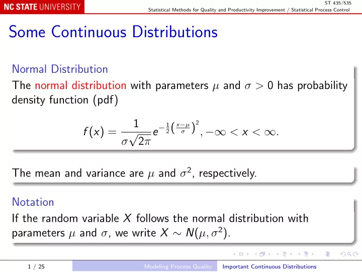
ST 435/535 Statistical Methods for Quality and Productivity Improvement / Statistical Process Control The standard normal distribution has µ = 0 and σ = 1, and pdf 1 e − 1 2 x 2 , −∞ < x < ∞ . ϕ ( x ) = √ 2 π The cumulative distribution function (cdf) of the standard normal distribution is � x Φ( x ) = ϕ ( y ) dy −∞ It cannot be written in closed form, but can be computed or tabulated. 2 / 25 Modeling Process Quality Important Continuous Distributions

ST 435/535 Statistical Methods for Quality and Productivity Improvement / Statistical Process Control Linear transformation If X has a normal distribution, say X ∼ N ( µ, σ 2 ), and Y = a + bX for some constants a and b , then Y is also normally distributed. By the basic rules of expected values, Y has mean a + b µ and variance b 2 σ 2 , so Y ∼ N ( a + b µ, b 2 σ 2 ). 3 / 25 Modeling Process Quality Important Continuous Distributions

ST 435/535 Statistical Methods for Quality and Productivity Improvement / Statistical Process Control Standardizing a random variable If X ∼ N ( µ, σ 2 ), then Z = X − µ σ has mean 0 and variance 1, so Z ∼ N (0 , 1), and P ( Z ≤ z ) = Φ( z ) . So � Z ≤ x − µ � � x − µ � P ( X ≤ x ) = P = Φ σ σ We use calculations of Φ( · ) to make probability statements about X by standardizing X into Z . 4 / 25 Modeling Process Quality Important Continuous Distributions

ST 435/535 Statistical Methods for Quality and Productivity Improvement / Statistical Process Control Example The time X to resolve a customer complaint at a certain financial institution is normally distributed with mean µ = 40 hours and standard deviation σ = 2 hours. How many complaints are resolved in at most 35 hours? � Z = X − 40 ≤ 35 − 40 � P ( X ≤ 35) = P = − 2 . 5 2 2 = Φ( − 2 . 5) = 0 . 00621 . Use the table in Appendix II or the R function pnorm(-2.5) to find the value 0 . 00621. So fewer than 1% of complaints are resolved in 35 hours or less. 5 / 25 Modeling Process Quality Important Continuous Distributions

ST 435/535 Statistical Methods for Quality and Productivity Improvement / Statistical Process Control Example, continued How long do 95% of complaints take to be resolved? 0 . 95 = P ( Z ≤ 1 . 645) = P (40 + 2 Z ≤ 40 + 2 × 1 . 645) = P ( X ≤ 43 . 29) . Use inverse look-up in the same table, or the R function qnorm(0.95) , to find the value 1 . 645. So 95% of complaints are resolved in 43 . 29 hours or less. 6 / 25 Modeling Process Quality Important Continuous Distributions

ST 435/535 Statistical Methods for Quality and Productivity Improvement / Statistical Process Control Central Limit Theorem Why is the normal distribution used as a model for data variation? The Central Limit Theorem (CLT) implies that any variable that is the accumulation of many small contributions is close to normal. Specifically: if X 1 , X 2 , . . . , X n are independent random variables with means µ i and variances σ 2 i , and if Y n = X 1 + X 2 + · · · + X n , then the distribution of Z n = Y n − � n i =1 µ i �� n i =1 σ 2 i approaches the standard normal distribution as n approaches infinity. Note Some constraints on the variances and on the tails of the distributions are needed for the CLT to hold. 7 / 25 Modeling Process Quality Important Continuous Distributions

ST 435/535 Statistical Methods for Quality and Productivity Improvement / Statistical Process Control Lognormal distribution If X is a positive random variable, and W = log X ∼ N ( θ, ω 2 ), then X has the lognormal distribution with parameters θ and ω . The mean and variance of X are E( X ) = e θ + 1 2 ω 2 and e ω 2 − 1 e 2 θ + ω 2 = e ω 2 − 1 � � � � E( X ) 2 . Var( X ) = Sometimes used as a model for the time-to-failure of a piece of equipment. 8 / 25 Modeling Process Quality Important Continuous Distributions

ST 435/535 Statistical Methods for Quality and Productivity Improvement / Statistical Process Control Exponential distribution The pdf of the exponential distribution is f ( x ) = λ e − λ x , x ≥ 0 where λ > 0 is the rate parameter of the distribution. The mean and variance are E( X ) = 1 λ and Var( X ) = 1 λ 2 . 9 / 25 Modeling Process Quality Important Continuous Distributions

ST 435/535 Statistical Methods for Quality and Productivity Improvement / Statistical Process Control The cdf is � x λ e − λ y dy = 1 − e − λ x , F ( x ) = P ( X ≤ x ) = 0 and P ( X > x ) = 1 − F ( x ) = e − λ x . 10 / 25 Modeling Process Quality Important Continuous Distributions

ST 435/535 Statistical Methods for Quality and Productivity Improvement / Statistical Process Control Lack of memory If x ′ > 0, then P ( X ≤ x + x ′ | X > x ) = F ( x + x ′ ) − F ( x ) 1 − F ( x ) = e − λ x − e − λ ( x + x ′ ) e − λ x = 1 − e − λ x ′ . That is, conditionally on X > x , the distribution of X − x is the same as the unconditional distribution of X : “lack of memory”. 11 / 25 Modeling Process Quality Important Continuous Distributions

ST 435/535 Statistical Methods for Quality and Productivity Improvement / Statistical Process Control Suppose you are waiting for a bus that runs on average every 10 minutes. If the time until the arrival of the next bus is exponentially distributed, the expected waiting time is 10 minutes. If no bus arrives in the first 5 minutes (or 10 minutes, or ...), the expected waiting time is still a further 10 minutes. 12 / 25 Modeling Process Quality Important Continuous Distributions

ST 435/535 Statistical Methods for Quality and Productivity Improvement / Statistical Process Control Also, if x ′ is small, P ( X ≤ x + x ′ | X > x ) ≈ λ x ′ . When X is time-to-failure of some system, λ is the failure rate of the system. In words: P (fail in a short time interval | not failed at the start) ≈ failure rate × length of interval . 13 / 25 Modeling Process Quality Important Continuous Distributions

ST 435/535 Statistical Methods for Quality and Productivity Improvement / Statistical Process Control Gamma distribution The pdf of the gamma distribution is λ Γ( r )( λ x ) r − 1 e − λ x , x > 0 f ( x ) = where r > 0 is the shape parameter and λ > 0 is the rate parameter . The special case r = 1 is the exponential distribution. Warning Montgomery calls λ the scale parameter, but the scale of the distribution is really 1 /λ . 14 / 25 Modeling Process Quality Important Continuous Distributions

ST 435/535 Statistical Methods for Quality and Productivity Improvement / Statistical Process Control The mean and variance are E( X ) = r λ and Var( X ) = r λ 2 . If r is an integer and X 1 , X 2 , . . . , X r are independent exponential random variables with rate parameter λ , then X = X 1 + X 2 + · · · + X r has the gamma distribution with shape parameter r and rate parameter λ . Also known as the Erlang distribution . 15 / 25 Modeling Process Quality Important Continuous Distributions

ST 435/535 Statistical Methods for Quality and Productivity Improvement / Statistical Process Control Weibull distribution The pdf of the Weibull distribution is f ( x ) = β � x � β − 1 � � x � β � exp − , θ θ θ where β > 0 is the shape parameter and θ > 0 is the scale parameter. The mean and variance are, forgettably, � � 1 + 1 E( X ) = θ Γ β and � �� 2 � � 1 + 2 � � � 1 + 1 Var( X ) = θ 2 Γ − Γ . β β 16 / 25 Modeling Process Quality Important Continuous Distributions

ST 435/535 Statistical Methods for Quality and Productivity Improvement / Statistical Process Control The cdf is � � β � � x F ( x ) = 1 − exp − . θ If Y follows the exponential distribution with rate parameter 1, and X = θ Y 1 /β , then � � β � � x P ( X ≤ x ) = 1 − exp − , θ so X follows the Weibull distribution. 17 / 25 Modeling Process Quality Important Continuous Distributions

ST 435/535 Statistical Methods for Quality and Productivity Improvement / Statistical Process Control The Weibull distribution is also used to model time-to-failure, with failure rate β � x � β − 1 . θ θ If β > 1, the failure rate increases over time, while if β < 1 the failure rate decreases over time. The special case β = 1 is the exponential distribution, with constant failure rate. 18 / 25 Modeling Process Quality Important Continuous Distributions